To compute MHD-waves along magnetic flux tubes one can again use a simple 1D time-dependent radiation-hydrodynamic code where the tube model is pictured as a stack of mass elements that are connected but can individually move in three dimensions. This so-called thin flux-tube approximation, where the physical variables do not vary much over the tube cross-section and are given by the values at the tube center, is a very simple approximation and gives reasonable results compared to a more realistic treatment of the flux tube (Hasan & Ulmschneider 2004a, b). The waves are introduced at the bottom of the tube by specifying different types of longitudinal or transverse velocities on basis of the given wave energy flux and the assumed wave period.

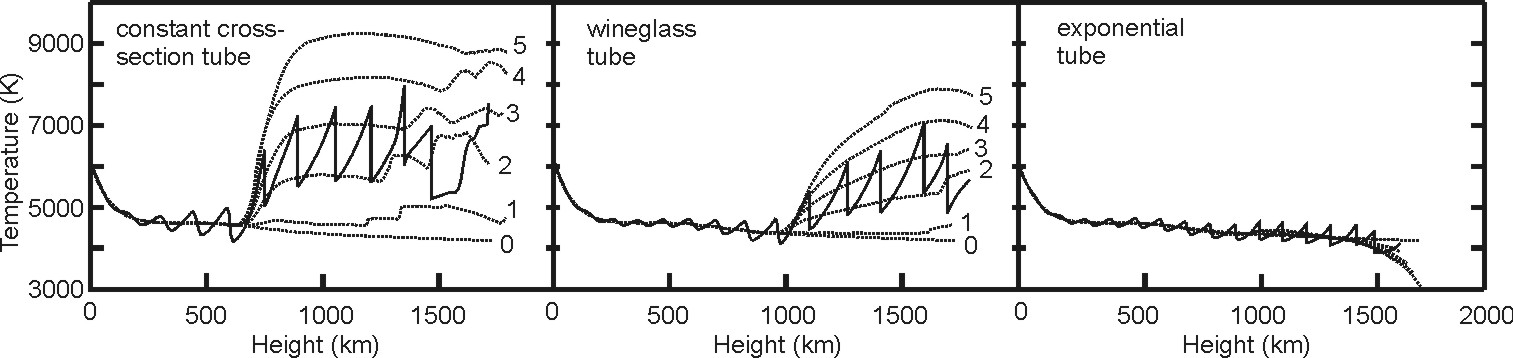
The heating of magnetic tubes does not only depend on the available wave energy flux but also on the spreading of the tube, that is, on how quickly the tube cross-section increases with height. In Fig. 8 from Fawzy, Ulmschneider & Cuntz (1998) it is seen that for three tubes of different geometry the shock dissipation behaves differently. These tubes have the same cross-section at the bottom, the same wave energy input, and the same wave period of 20 s. There essentially is no heating in the exponential tube because the available wave energy is spread over a rapidly increasing cross-section and only very weak shocks form.

The constant cross-section tube has maximum heating. The wineglass tube geometry, which at at 1300 km height reaches a constant cross-section, is the most realistic case for magnetic regions. This maximum cross-section at the top of the tube is enforced by the other tubes which surround an individual tube. Since all tubes spread with height, they can only spread until all the available space is filled. Therefore, for a specified filling factor f the spreading of the flux tube model (Fig. 5) is important for the predicted wave heating.

Fig. 8 Shock wave heating by an adiabatic wave of period 20 s in magnetic flux tubes of different geometry: Constant cross-section tube (left), wine glass tube (center), exponentially spreading tube (right). Mean values from 0 to 5 are shown dotted in 400 s intervals, after Fawzy, Ulmschneider & Cuntz (1998)

To compare the chromosphere of a magnetic star with observations one has to simulate the core emission of the Ca II and Mg II lines. The flux tube geometry on stars with different filling factors and the ray paths used in the computation of the emergent intensity is shown in Fig. 9.

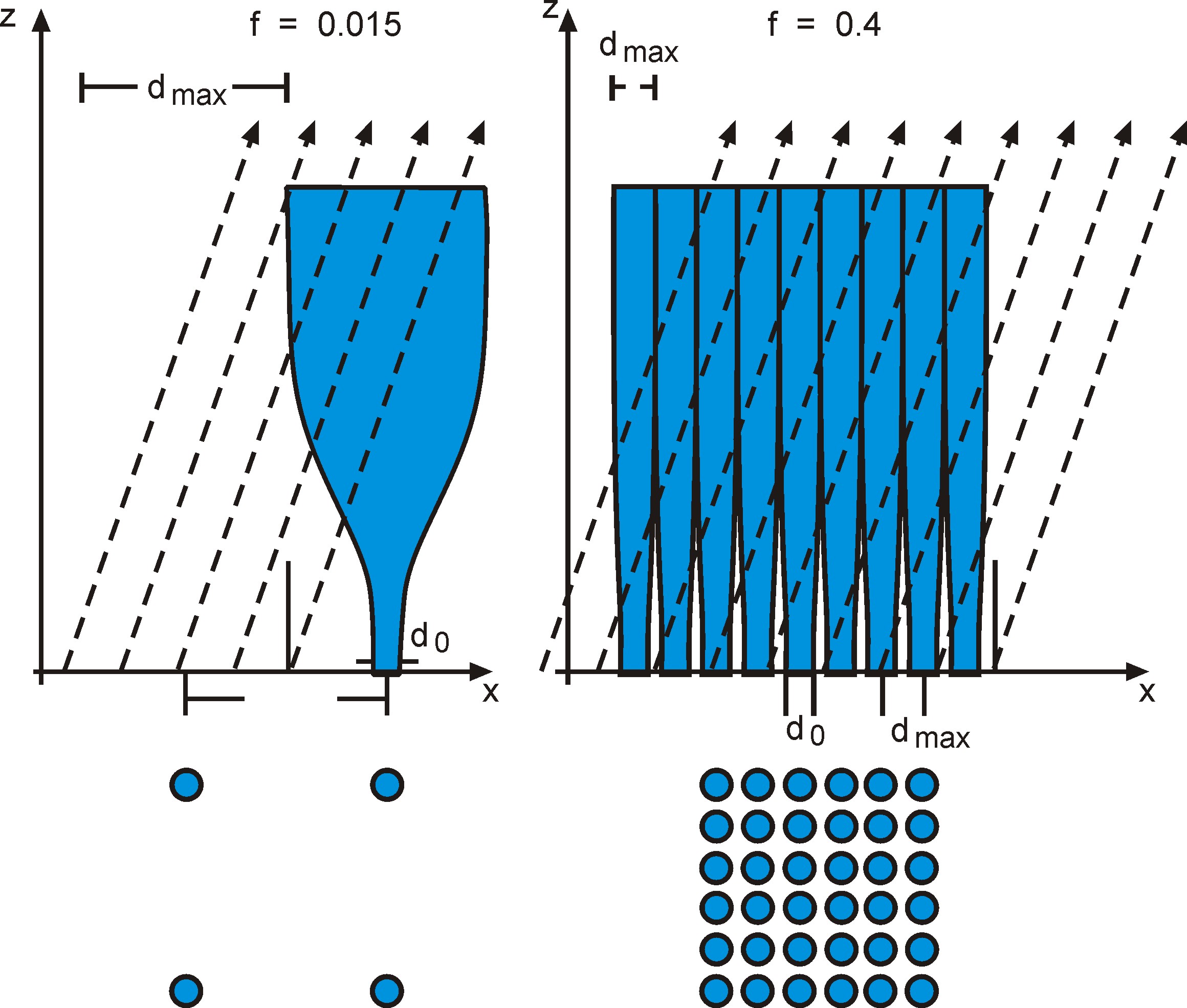
Fig. 9 Ray-paths through the forest of flux tubes for the computation of the emergent line radiation from stars with different magnetic filling factors f, after Cuntz et al. (1999) and Fawzy et al. (2002b). The arrangement of the tube cross-sections on the stellar surface is shown at the bottom

For a first application of our MHD-wave heating picture of magnetic chromospheres we selected K0V to K3V main sequence stars as a test case where the relationship between the magnetic flux and the rotation period, that is, the filling factor f as function of P_{Rot}, is known from observations. There are two effects that affect the heating in stars of the same spectral type but different rotation periods. The magnetic field strength B at the stellar surface on the stars in every flux tube is the same because it is related to the gas pressure at the stellar surface which does not change with P_{Rot}, but the number of tubes and the amount of spreading is different (see Fig. 5). For each star we therefore have a flux tube model with the same cross-section at the stellar surface but different spreading in which the same computed longitudinal wave energy flux is introduced. We also assume that 10% of the transverse wave flux is converted to longitudinal wave flux due to mode-coupling.

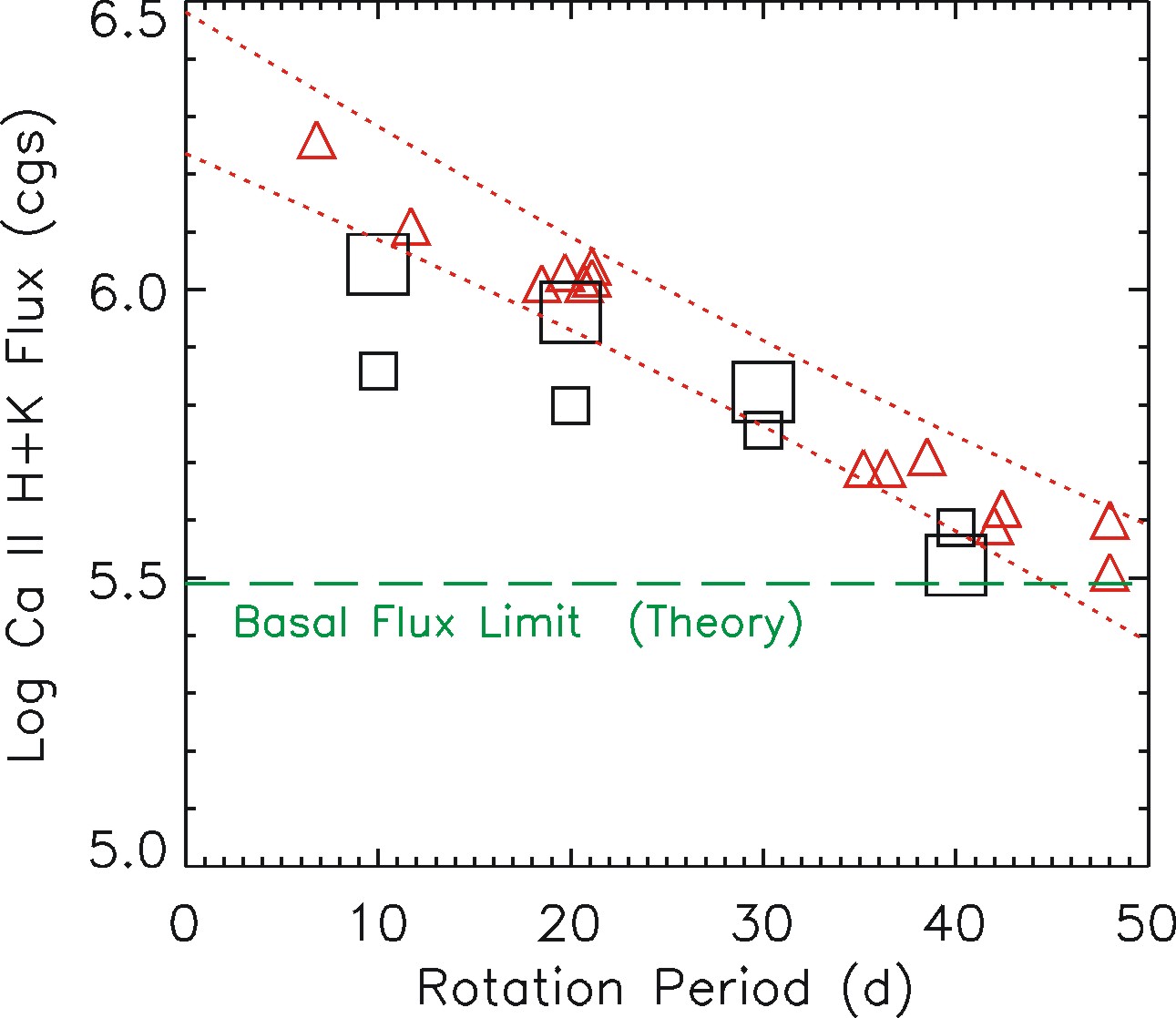
Fig. 10 Ca II H+K emission flux as function of stellar rotation, after Cuntz et al. (1999). The triangles give the observations for a set of stars with spectral type between K0V and K3V, which constitutes the empirical rotation-chromospheric emission relation. The squares indicate the results from two-component theoretical chromosphere models. The basal flux limit from pure acoustic heating is indicated

Figure 10 shows the comparison of our simulations with observations for the Ca II H+K line core emission (Cuntz et al. 1999). It is seen that the observed rotation-chromospheric emission correlation is reasonably well reproduced. This may indicate that we have correctly identified the magnetic heating mechanism of chromospheres as MHD-waves.

For a more reliable identification of the MHD-wave heating picture of magnetic chromospheres this type of approach was carried out for many other stars and spectral lines (Ulmschneider et al. 2001, Fawzy et al. 2002a, b, c). Figure 11 shows the simulated Ca II core emission based on MHD-wave heating for main sequence stars of different assumed filling factors f with observations. It is seen that with increasing f the observed range between the basal flux limit and the saturation limit is essentially covered. Here we have limited f at a maximum value of f = 0.4 because as seen in Fig. 9 the flux tubes for that case still leave enough non-magnetic external space in the convection zone for the external turbulent motions to generate the MHD-wave energy. Since for higher values of f the convective motions and therefore the MHD-wave generation are thought to be impared, the case f approx 0.4 should give the maximum MHD-wave generation in stars.

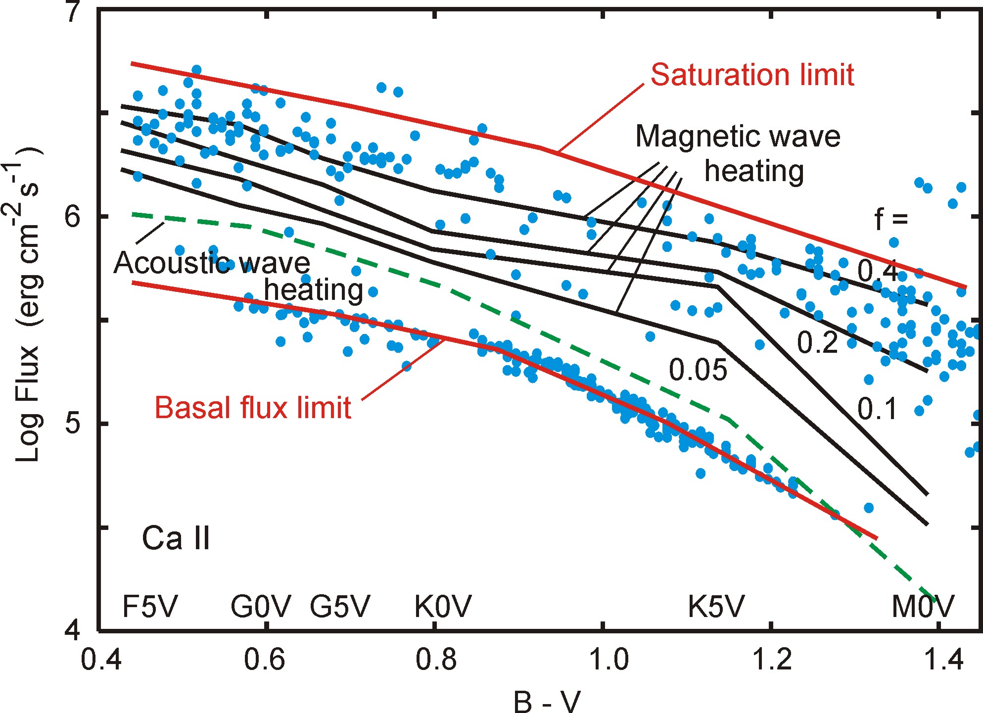
Fig. 11 Observed chromospheric Ca II H+K line core emission fluxes of individual stars compared with theoretical simulations based on MHD-wave heating in stars covered by different amounts of magnetic flux specified by the magnetic filling factor f, after Fawzy et al. (2002b)

Figures 12 and 13 show for the Ca II H+K and Mg II h+k lines the maximum MHD-wave heating with filling factors f = 0.4 but different amounts of transverse wave heating added on top of the longitudinal wave heating. Since the transverse wave energy fluxes are much higher than the longitudinal wave fluxes we have multiplied the longitudinal fluxes by a factor M to take into account the conversion of transverse wave energy to longitudinal energy by mode-coupling. It is seen that the additional energy does not change the picture much. If we trust our crude methods it can be seen that while the Ca II saturation limit is reasonably well reproduced there seems to be a heating gap for the Mg II saturation limit. This may be due to our simple approach or could point to the neglected heating by magnetic field reconnection. This latter heating mechanism is supposed to become more important in higher layers (compared to the Ca II formation heights) where the Mg II line cores are formed and particularly in the corona. Another reason might be the crude handling of the mode-coupling with the much more energetic transverse waves.

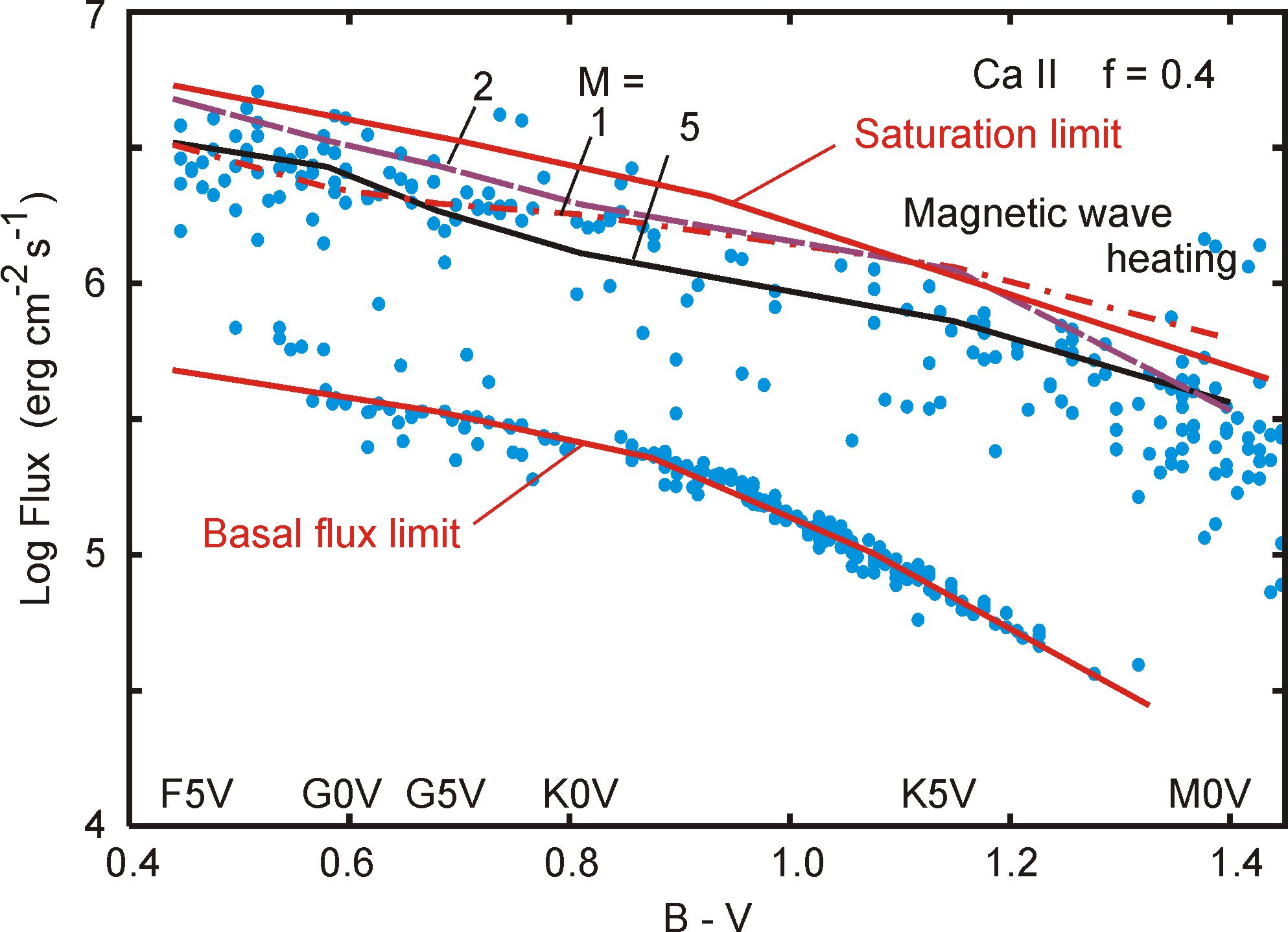
Fig. 12 Ca II H+K emission core flux observations in comparison with theoretical simulations with different amounts of maximum wave energy present when the magnetic filling factor is f = 0.4. Mode-coupled transverse wave energy is assumed to increase the longitudinal wave flux by the indicated factors M, after Fawzy et al. (2002b)

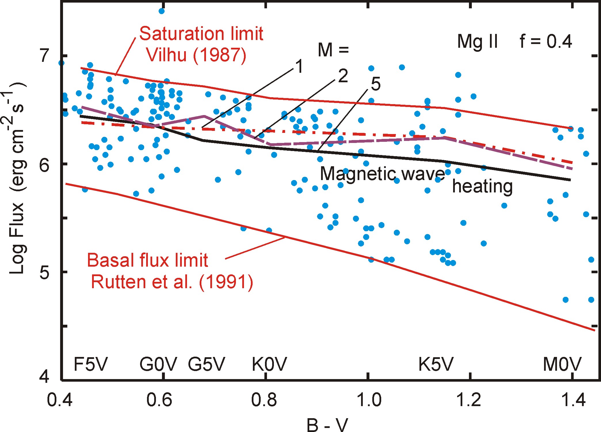
Fig. 13 Mg II h+k emission core observations in comparison with theoretical simulations with different amounts of maximum wave energy present when the magnetic filling factor is f=0.4. Mode-coupled transverse wave energy is assumed to increase the longitudinal wave flux by the indicated factors M, after Fawzy et al. (2002b)