
Visualization techniques
Visualization of turbulent motion in the jet cocoon
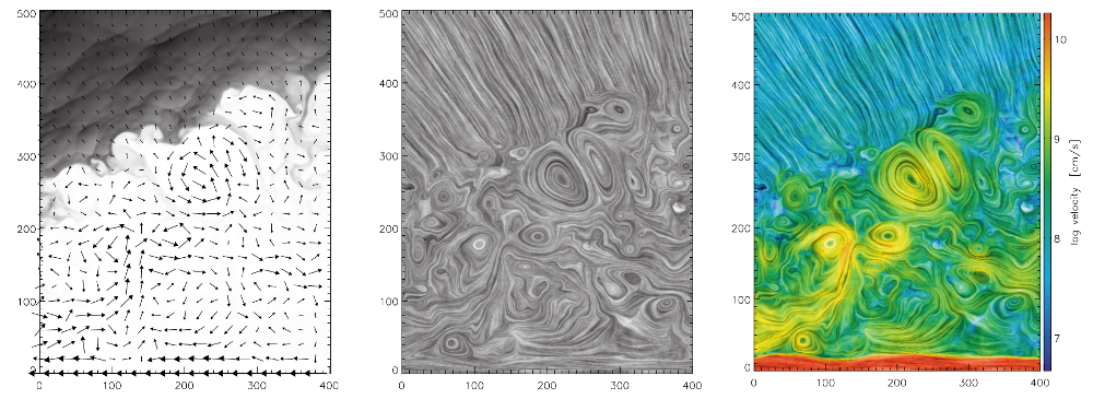
While visualization of 2D scalar fields can easily be done by using color maps, the traditional approach for vector fields is to use arrows pointing in direction of the vector fields. This gives a reasonable representation for ordered fields, but is mostly useless for turbulent vector fields or fields with small-scale structures. Line Integral Convolution (LIC) was described by Cabral & Leedom (1993) and is based on computation of stream lines. It gives a representation similar to iron filing on a paper tracing the field lines of a magnet. Each pixel in the LIC image is obtained by integrating over a white noise image along a streamline of certain length through the respective pixel position, and writing the result to that pixel. The stream line is computed from the vector field array aligned with the noise image. Vector field, noise field and output field need to have the same size for this. Often a constant integration kernel (averaging) is used, but other kernels can be chosen at will (e.g. increasing weight in direction of the vector field). Furthermore, the noise image can be replaced by any other image or pattern, which is then blurred in direction of the vector field.
 Due to a large number of stream lines to be computed, LIC is rather
computationally demanding. However, current computers are fast enough for
this and the method is easily parallelizable. Though this technique is
already 15 years old, it has not been, to my knowledge, included in any
general-purpose visualization software yet.
Due to a large number of stream lines to be computed, LIC is rather
computationally demanding. However, current computers are fast enough for
this and the method is easily parallelizable. Though this technique is
already 15 years old, it has not been, to my knowledge, included in any
general-purpose visualization software yet.
LIC images, however, do not contain information about the vector field magnitude. To add this, we extended the method to represent the field magnitude by colors: working in HLS (hue–lightness–saturation) color space instead of RGB (red–green–blue) the LIC image was encoded as lightness and the field magnitude as hue value (color). Saturation could be used, theoretically, to encode another field, but in practice this is not perceived well enough by the human eye to add any real value. Similar results could be achieved by adding or multiplying the LIC field and the magnitude scalar field and displaying it with a usual color scale, but here it might occur that stream line and magnitude contribution can not be disentangled anymore, while for the HLS approach the information is clearly separate. To account for difficulties in distinguishing colors for high or low brightness, the lightness parameter should be limited in range (e.g. [0.05, 0.95]) and the saturation value should be somewhat lower than unity (e.g. 0.8).
The figure here shows the comparison of an arrow plot and the LIC representations. For arrow plots, usually arrow lengths are chosen to be proportional to the field magnitude. Since the field magnitude varies by more than two orders of magnitude, only arrows within the beam (shown red in the color LIC image) were visible then. For the present case of jet simulations, the arrow plot uses an asinh function applied to the arrow lengths, resulting in a logarithmic- like display of the field strength, where even slow moving regions are easily recognizable. Yet it is evident that the LIC images show much more flow details than possible with arrows. This is even more drastic for images showing only part of the flow with relatively large vortices but the whole computational domain, where vortex sizes generally will be much smaller than spatial resolution of the arrows. For largely varying field magnitudes, it is however very important to include the magnitudes to be able to judge the “importance” of motion, as possible with our color LIC images.
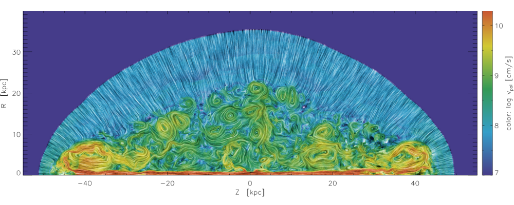
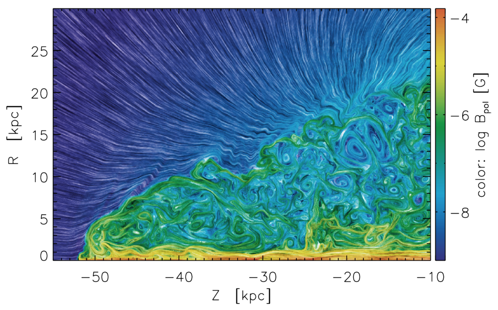
The figures below shows an application of the method. One shows the poloidal
velocity component for a magnetized jet with density contrast
0.001. The backflow and large vortices are produced in the jet head and
then cascade down towards a turbulent spectrum in the jet cocoon. In the other,
the poloidal magnetic field is shown. Outside the jet cocoon, it is weak and
nicely ordered, while the inside is dominated by vortices and a strong poloidal
field in the jet beam.
It is important to mention that there is still a limitation with this representation: direction of the flow (forward vs. backward) cannot be displayed with LIC images. While use of asymmetric kernels (e.g. linearly increasing in direction of the flow) may include this information, this was found to be only of limited use for turbulent fields with their fine-grained structures; direction of the flow, though, is not very important in this case due to the stochastic nature of turbulent patterns, and regions of well-ordered flow (beam and shocked ambient gas) have directions which are already clear from the physical setup. If directional information were important, the LIC images would have to be supplemented by arrow plots. Image-guided stream lines (OSTR, Turk & Banks, 1996; Laidlaw et al., 2001) might then provide a compromise between arrow plots and stream line techniques as LIC.
Science results: Gaibler et al. 2009
Visualization: Gaibler & Camenzind 2009
If you are interested in the code to generate the images, please contact me
via email.
Time-regridding for simulations movies
tbd.