Octree AMR models
Notes on octree AMR models
Models with octree mesh refinement are set up in a more or less similar way as models with regular grid with two fundamental key differences.
- Model function signature
For regular grids any model function(e.g. getDustDensity(), getGasTemperature(), etc) has the generic signature:
def func(grid=None, ppar=None)
Where grid is an instance of radmc3dGrid and ppar is a dictionary containing all parameters of the model. For octree AMR compatible
models the model functions have three additional arguments:
def func(x=None, y=None, z=None, grid=None, ppar=None)
where x, y, and z are arrays containing the cell center coordinates. The reason for the separate cell centre coordiante input is that it makes it simpler
to call model functions during grid building if the refinement criterion depends on the physical structure of the grid (e.g. density). As of radmc3dPy v0.29 both forms of
coordinate input is used (x, y, z and grid), however in future versions the grid argument might be removed.
- Decision function
Another important difference between models using regular and octree mesh is that the building of an octree grid requires a decision function to tell when cells should
be refined. It receives the cell centre coordinates and sizes as numPy ndarrays and returns a linear array of the same length containing boolean True or False values,
True if a cell should be refined and False if it should not. An example function based on the gas density gradient is implemented in
decisionFunction() of the ppdisk_amr model:
def decisionFunction(x=None, y=None, z=None, dx=None, dy=None, dz=None, model=None, ppar=None, **kwargs):

    ncell   = x.shape[0]
    rho     = np.zeros([ncell, kwargs['nsample']], dtype=np.float64)

    for isample in range(kwargs['nsample']):
        xoffset  = (np.random.random_sample(ncell)-0.5)*dx*4.0
        yoffset  = (np.random.random_sample(ncell)-0.5)*dy*4.0
        zoffset  = (np.random.random_sample(ncell)-0.5)*dz*4.0
        rho[:,isample] = model.getGasDensity(x+xoffset, y+yoffset, z+zoffset, ppar=ppar)

    rho_max = rho.max(axis=1)
    rho_min = rho.min(axis=1)
    jj      = ((rho_max-rho_min)/rho_max>ppar['threshold'])

    decision = np.zeros(ncell, dtype=bool)
    if True in jj:
        decision[jj] = True

    return decision
This function probes the gas density at a sample of random points within the cell \(\rho_{\rm i}\) and if the quantity \((\max{\rho_{\rm i}} - \min{\rho_\rm{i}})/\max{\rho_{\rm i}}\) is higher than a given threshold the cell is refined. The idea behind this refinement is to resolve sharp density transitions in the disk, i.e. the upper layers of the disk or the edges of possible gaps. Note, that the signature of a decision function is fixed to be:
def decisionFunction(x=None, y=None, z=None, dx=None, dy=None, dz=None, model=None, ppar=None, **kwargs)
This means that any other keyword argument should be passed to the function via **kwargs. Any extra keyword argument passed to the setup functions
(problemSetupDust() and problemSetupGas()) will be passed on to the decision function in the **kwargs
dictionary (and these keyword arguments will also be recorded in the problem_params.inp file).
The decision function for a model can be set in two ways. Either a function with a name of “decisionFunction” should be present in the model module next to the
usual model functions (just like in ppdisk_amr) or a function can also be passed to the setup functions
as a dfunc keyword argument. Finally, note that all AMR cell related arguments of a decision function (x, y, z, dx, dy, dz) can be numPy arrays.
Continuum model tutorial
Let us now see setp-by-step how this works in practice in a protoplanetary disk model implemented in ppdisk_amr.
This example can also be found in the python_examples/run_octree_amr_example_1 directory in the form of a single python script.
This example model is a slightly modified version of
the protoplanetary disk model ppdisk to be used with octree refined grids and the gaps in the disk are represented by a radial gaussian
instead of a step function. With the refinement decision function at hand we can generate a model where the grid is refined in the upper layers of the disk and the
edges of the gap while the resolution of the grid in the constant background density remain low.
Similar to the regular grid version we can start by creating a directory for our model and copy the dustkappa_silicate.inp file from the python_examples/datafiles
directory and start a python session.
First we import the radmc3dPy package:
from radmc3dPy import *
then create an input parameter file with the default parameters:
>>> analyze.writeDefaultParfile('ppdisk_amr')
Writing problem_params.inp
Now we can create the necessary input files for a dust continuum model:
>>> setup.problemSetupDust(model='ppdisk_amr', nsample=30, threshold=0.9, binary=False)
Writing problem_params.inp
Writing problem_params.inp
Adaptive Mesh Refinement (AMR) is active
Active dimensions : 0 1 2
Resolving level 0
Cells to resolve at this level :  200
Resolving level 1
Cells to resolve at this level :  1170
Resolving level 2
Cells to resolve at this level :  7394
Resolving level 3
Cells to resolve at this level :  46193
Resolving level 4
Cells to resolve at this level :  266083
Tree building done
Maximum tree depth :  5
Nr of branches     :  321040
Nr of leaves       :  2247496
Generating leaf indices
Done
Writing dustopac.inp
Writing wavelength_micron.inp
Writing amr_grid.inp
Writing stars.inp
-------------------------------------------------------------
Luminosities of radiation sources in the model :
As calculated from the input files :
Stars :
  Star #0 + hotspot        : 3.564346e+33
Continuous starlike source : 0.000000e+00

-------------------------------------------------------------
Writing dust_density.inp
Writing radmc3d.inp
This is now a bit different from a model setup with regular grids. First we passed two extra keyword argument to the dust setup function, which are
required by the cell refinement decision function. nsample=30 sets the number of random location within the cell to be used to estimate the density
structure of the model within a given cell while threshold=0.9 sets the lower limit for \((\max{\rho_{\rm i}} - \min{\rho_\rm{i}})/\max{\rho_{\rm i}}\)
above which the cell should be refined.
In the output we will see how many cells get refined at each level and the maximum level of refinement in the model. We can limit the depth of the grid, i.e.
the highest refinement level with the levelMaxLimit parameter in the problem_params.inp file or as a keyword argument in the call of the setup function.
We also get the information on the number of branch and leaf nodes in the grid.
Read the model structure
We have generated a dust model but now we should look at it whether it is really what we intended to have. Using simple 2D plotting functions in matplotlib it
is not possible to display data defined at a random, irregularly spaced points. There are possibilities, though like the tripcolor() or tricontourf() functions,
but they tend to show some artifacts at the edges of the grid, which can lead to confusion in interpreting these plots. Thus a better way is to regrid the data to a regular mesh
and do the visualisation of the regridded data. radmc3dPy has a new function plotSlice2D() that makes it simple to plot any axis-aligned
2D slices of the model. It works with models using both regular or octree AMR grids. For octree grids it uses the interpolateOctree()
function to do nearest neighbour interpolation to a regular grid. To create a plot of the vertical density structure of the model we need to read the density
first:
>>>d = analyze.readData(ddens=True, octree=True, binary=False)
This tells radmc3dPy to read the dust density from a model using octree where the format of the dust density input file is formatted ascii. Apart from the dust density it also reads the spatial grid. The reading of the spatial grid takes more time than reading the density file or possibly even slower than creating the grid. The reason for this is that when the spatial grid is read from the file at each base grid cell we immediately follow the tree and add refinement to the nodes immediately before moving on to the next base grid cell. As discussed above in Grid building this is the slower way of building an octree mesh in python. During grid building therefore we use array operations to process to test and refine all cells at a given level, which is significantly faster.
To save time on reading the grid and speed up data reading there are two options. One possibility is that we use the data reading methods of
radmc3dData. For instance, we have read the dust density, but if we additionally want to read the dust temperature as well we can use
readDustTemp():
>>>d.readDustTemp(binary=False, octree=True)
The other possibility is if we pass the instance of the radmc3dOctree or radmc3dGrid to the
readData function. If we have already read the grid contained in the instance g then we can pass it on to the data reader
function to use this grid instead of readin it from file:
>>>d = analyze.readData(ddens=True, octree=True, binary=False, grid=g)
Diagnostic plots
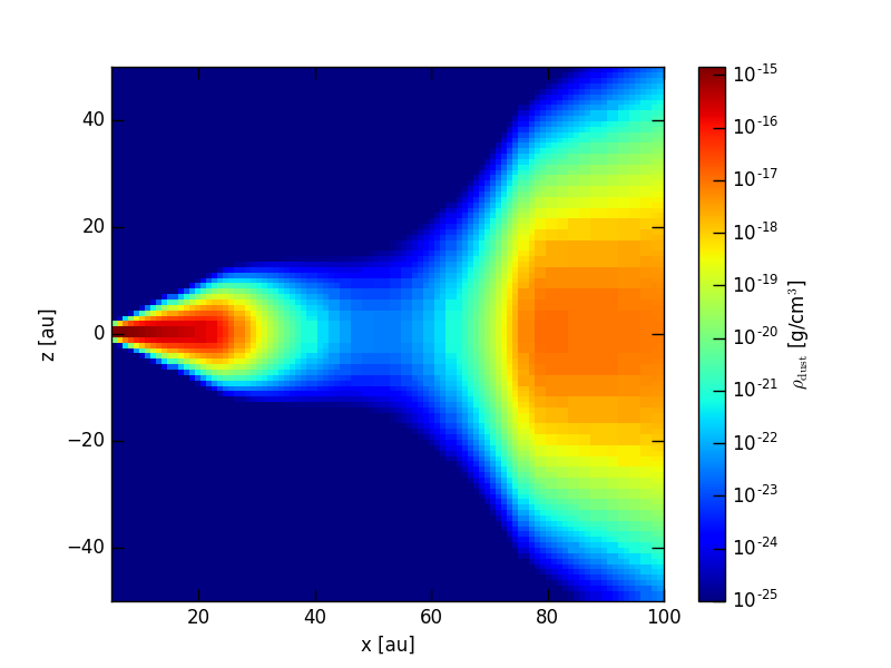
After we have read the grid and the density structure we can use plotSlice2D() to create a plot of the density structure in our model:
>>>analyze.plotSlice2D(data=d, plane='xz', var='ddens', showgrid=False, linunit='au',
       nx=100, ny=100, xlim=(5., 100.), ylim=(-50., 50.), log=True, vmin=1e-25,  nproc=3)
This command plots the density structure (var='ddens') along in the vertical plane (plane='xy', the order of the cooridinates matters),
using AU as the unit of any linear axis of the plot (linunit='au') using a regular grid between 5AU and 100AU in the x coordinate
(xlim=(5., 100.)) and between -50AU and 50AU in the z coordinate (ylim=(-50., 50.)) placing 100-100 pixels to create a regular
grid in the slice (nx=100, ny=100). The plot will use a logarithmic stretch (log=True) with a lower cut of 1e-25 for the density
(vmin=1e-25) and using three parallel processes for the interpolation (nproc=3). We should get an plot like this:
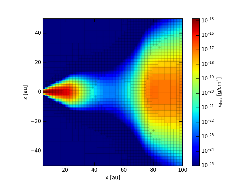
By adding the showgrid=True and gridalpha=0.1 keywords to the call of plotSlice2D() we can also display
the boundaries of the octree grid cells:
>>>analyze.plotSlice2D(data=d, plane='xz', var='ddens', showgrid=False, linunit='au', showgrid=True, gridalpha=0.1,
          nx=100, ny=100, xlim=(5., 100.), ylim=(-50., 50.), log=True, vmin=1e-25,  nproc=3)
which should result in a plot like this:
IMPORTANT: Since the refinement decision function works in a stochastic way, i.e. the refinement depends on the gas density taken at random location within the
grid cells, the resulting grid structure may change slightly from one run to another. To prevent the change of the grid in consecutive runs, one can do two things.
First, use a fixed seed number for the random number generator in the decision function and second, increase the number of density sampling points (nsample parameter).
Keep in mind, thought, that the higher the number of density sampling point, the slower the model setup will become.
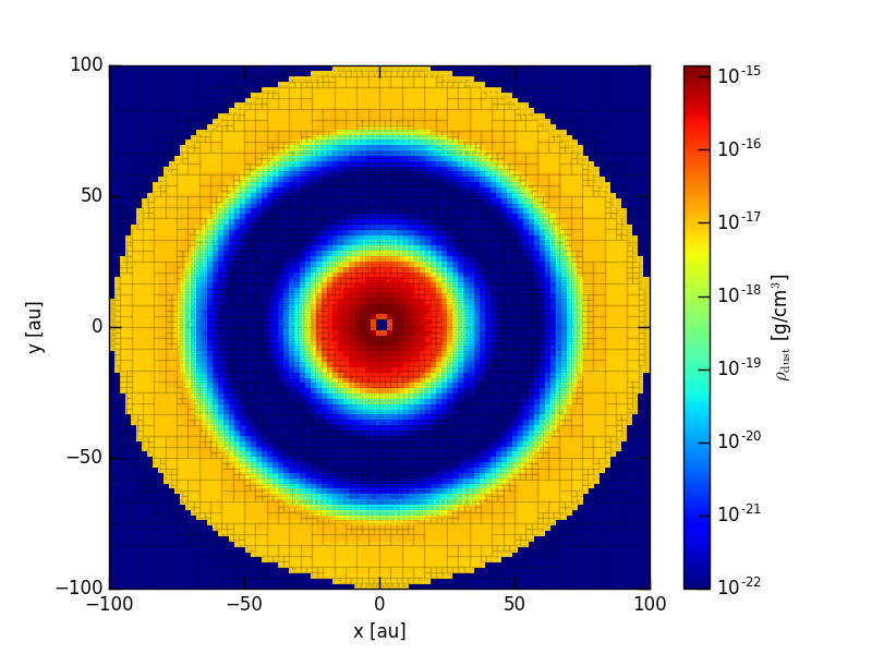
We can also plot a slice of the density structrue in the disk midplane, by setting plane='xy':
>>>analyze.plotSlice2D(data=d, plane='xz', var='ddens', showgrid=False, linunit='au', showgrid=True, gridalpha=0.1,
       nx=100, ny=100, xlim=(5., 100.), ylim=(-50., 50.), log=True, vmin=1e-25,  nproc=3)
which should result in a plot like this:
Once we are convinced that the density structure of the model is what we expect it to be we can calculate the dust temperature:
>>> import os
>>> os.system('radmc3d mctherm')
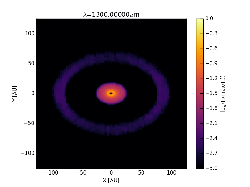
and also calculate a continuum image at \(\lambda=1300\,\mu m\):
>>> image.makeImage(npix=400, sizeau=250., incl=45., wav=1300.)
We can then read and display the image as:
>>> im = image.readImage()
>>> image.plotImage(im, au=True, log=True, maxlog=3, cmap=plt.cm.inferno)
resulting in an image like this
Line model tutorial
Setting up a gas model is now really simple. Since we have already dealt with the creatin of the spatial grid we can call the gas setup function in the exact same way as in the case of a regular grid:
>>> setup.problemSetupGas(model='ppdisk_amr', binary=False)
The molecular number density, gas velocity and microturbulent velocity fields are now created for the default molecule of carbon-monoxide.
To calculate observables, images or spectra, we need to copy the molecular data file molecule_co.inp (LAMBDA format) from the datafiles
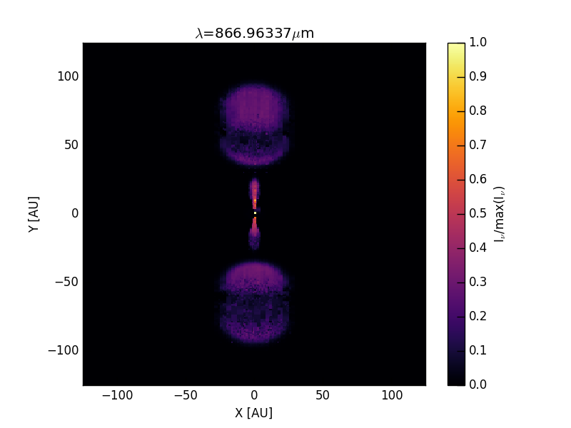
directory to the current model directory. Then we are ready to calculate a channel map of the J=3-2 transition at zero velocity:
>>> image.makeImage(npix=400, sizeau=250., incl=45., iline=3, vkms=0.)
We can then display this image:
>>> im = image.readImage()
>>> image.plotImage(im, au=True, cmap=plt.cm.inferno)
We should then get an image like this: