Line model tutorial (regular grid)

Model setup

Similarly to the dust setup we can use the problemSetupGas() method to create all necessary input files for the line simulations. In the following we will take the protoplanetary disk model as an example. It requires the dust model setup to be complete and the dust temperature to be calculated (to set up a simple abundance model with photodissociation and freeze-out). To enhance the effect/visibility of the freeze-out of the molecules close to the midplane rise the freeze-out temperature to 40K (Note, the real freeze-out temperature of CO molecules is around 19K and the 40K used here is only for illustration purpose):

>>> setup.problemSetupGas('ppdisk', gasspec_mol_freezeout_temp=[40.])

The problemSetupGas() method takes one mandatory argument, the name of the model. Let us now see the gas structure in the disk. First we need to read the gas density:

>>> data = analyze.readData(gdens=True, ispec='co')

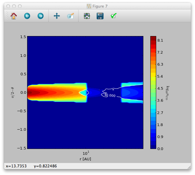
The readData() method reads the content of the molecule_co.inp and puts it into the radmc3dData.ndens_mol attribute. When reading gas density with the readData() method we always need to specify the name of the species with the ispec keyword (i.e. the part of the filename between molecule_ and .inp). We can now make contour plots to display a vertical slice of the disk:

>>> sc = plb.contourf(data.grid.x/natconst.au, np.pi/2.-data.grid.y, np.log10(data.ndens_mol[:,:,0,0].T).clip(1e-3), 30)
>>> splb.xlabel('r [AU]')
>>> splb.ylabel(r'$\pi/2-\theta$')
>>> splb.xscale('log')
>>> scb = plb.colorbar(c)
>>> scb.set_label(r'$\log_{10}{n_{\rm CO}}$', rotation=270.)

We can also overplot the dust temperature to check whether freeze-out really happens at 40K as we specified:

>>> data.readDustTemp()
>>> sc = plb.contour(data.grid.x/natconst.au, np.pi/2.-data.grid.y, data.dusttemp[:,:,0,0].T, [40.],  colors='w', linestyles='solid')
>>> splb.clabel(c, inline=1, fontsize=10)

The result should look like this:

Images

To calculate images/channel maps we need one additional data file with the molecular data (level energies, Einstein coefficients, etc.). Such files can be downloaded e.g. from the Leiden Atomic and Molecular Database. Note, that the files downloaded from the Leiden database need to be renamed to molecule_MOLECULENAME.inp (e.g. co.dat -> molecule_co.inp). For our example we can also use the molecule_co.inp (12C16O data file downloaded from the Leiden database) in the python_examples/datafiles directory and copy it to the model directory. Then we are ready to make line channel maps:

>>> image.makeImage(npix=300., incl=50., phi=0., sizeau=300., vkms=0.5, iline=3)

This command will calculate an image with 300 pixel and 300 AU each side, at an inclination of 50 degree. The image will be calculated for the third line/transition int the molecular data file at a frequency/wavelength corresponding to 0.5 km/s assuming zero systemic velocity for the source. To calculate a full 3D image qube with multiple frequencies/velocities at once, instead of the vkms keyword one can use the widthkms and linenlam keywords. The widthkms keyword will set the total width of the image qube in velocity (in the unit of km/s) while the linenlam keyword will set at how many linearly spaced velocity bins should images be calculated for that interval. For the details of how to calculate line channel maps see the RADMC-3D manual.

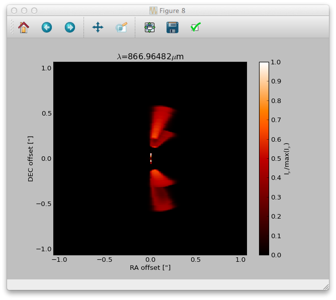
Now we can read the calculate image (channel map):

>>> im = image.readImage()

And display it

>>> image.plotImage(im, arcsec=True, dpc=140., cmap=plb.cm.gist_heat)