Continuum model tutorial (regular grid)
Model setup
First let us create a directory for our model. Then go to this directory and start python and
copy the dustkappa_silicate.inp file from the python_examples/datafiles directory to the
model directory. Then go to the model directory and start a python session.
Import the radmc3dPy package:
from radmc3dPy import *
This way we imported all core modules of the package: analyze, image,
setup, natconst.
The models module contains all models (like a library). To check what models are available
we can use the getModelNames() function:
>>> models.getModelNames()
['lines_nlte_lvg_1d_1', 'ppdisk', ''disk_acc', 'ppdisk_amr', 'simple_1', 'sphere1d_1', 'sphere2d_1', 'test_scattering_1']
We can also get a brief description of any model with the getModelDesc() function:
>>> models.getModelDesc('ppdisk')
'Generic protoplanetary disk model'
To create a model, we need to have a master parameter file containing all parameters of the model.
Every model in the library has a default set of parameters which can be used to, e.g. test the model.
We can use this default parameterset to create the parameter file with the writeDefaultParfile()
function.:
>>> analyze.writeDefaultParfile('ppdisk')
Writing problem_params.inp
Then we can read the parameters from this file...:
>>> par = analyze.readParams()
... and print them:
>>> par.printPar()
# -------------------------------------------------------------------------------------------------------------------------
# Block: Radiation sources
# -------------------------------------------------------------------------------------------------------------------------
incl_cont_stellarsrc      = False  # # Switches on (True) or off (False) continuous stellar sources )
incl_disc_stellarsrc      = True  # # Switches on (True) or off (False) discrete stellar sources)
mstar                     = [1.0*ms]  # # Mass of the star(s)
pstar                     = [0.0, 0.0, 0.0]  # # Position of the star(s) (cartesian coordinates)
rstar                     = [2.0*rs]  # # Radius of the star(s)
staremis_type             = ["blackbody"]  # # Stellar emission type ("blackbody", "kurucz", "nextgen")
tstar                     = [4000.0]  # # Effective temperature of the star(s) [K]
# -------------------------------------------------------------------------------------------------------------------------
# Block: Grid parameters
# -------------------------------------------------------------------------------------------------------------------------
crd_sys                   = 'sph'  # Coordinate system used (car/cyl)
nw                        = [19, 50, 30]  # Number of points in the wavelength grid
nx                        = [30,50]  # Number of grid points in the first dimension
ny                        = [10,30,30,10]  # Number of grid points in the second dimension
nz                        = 0  # Number of grid points in the third dimension
wbound                    = [0.1, 7.0, 25., 1e4]  # Boundraries for the wavelength grid
xbound                    = [1.0*au,1.05*au, 100.0*au]  # Boundaries for the x grid
xres_nlev                 = 3  # Number of refinement levels (spherical coordinates only
xres_nspan                = 3  # Number of the original grid cells to refine (spherical coordinates only)
xres_nstep                = 3  # Number of grid cells to create in a refinement level (spherical coordinates only)
ybound                    = [0., pi/3., pi/2., 2.*pi/3., pi]  # Boundaries for the y grid
zbound                    = [0., 2.0*pi]  # Boundraries for the z grid
# -------------------------------------------------------------------------------------------------------------------------
# Block: Dust opacity
# -------------------------------------------------------------------------------------------------------------------------
dustkappa_ext             = ['silicate']  #
gdens                     = [3.6, 1.8]  # Bulk density of the materials in g/cm^3
gsdist_powex              = -3.5  # Grain size distribution power exponent
gsmax                     = 10.0  # Maximum grain size
gsmin                     = 0.1  # Minimum grain size
lnk_fname                 = ['/disk2/juhasz/Data/JPDOC/astrosil/astrosil_WD2001_new.lnk', '/disk2/juhasz/Data/JPDOC/carbon/A/cel600.lnk']  #
mixabun                   = [0.75, 0.25]  # Mass fractions of the dust componetns to be mixed
ngs                       = 1  # Number of grain sizes
# -------------------------------------------------------------------------------------------------------------------------
# Block: Gas line RT
# -------------------------------------------------------------------------------------------------------------------------
gasspec_colpart_abun      = [1e0]  # Abundance of the molecule
gasspec_colpart_name      = ['h2']  # Name of the gas species - the extension of the molecule_EXT.inp file
gasspec_mol_abun          = [1e-4]  # Abundance of the molecule
gasspec_mol_dbase_type    = ['leiden']  # leiden or linelist
gasspec_mol_name          = ['co']  # Name of the gas species - the extension of the molecule_EXT.inp file
# -------------------------------------------------------------------------------------------------------------------------
# Block: Code parameters
# -------------------------------------------------------------------------------------------------------------------------
istar_sphere              = 0  # 1 - take into account the finite size of the star, 0 - take the star to be point-like
itempdecoup               = 1  # Enable for different dust components to have different temperatures
lines_mode                = -1  # Line raytracing mode
modified_random_walk      = 0  # Switched on (1) and off (0) modified random walk
nphot                     = 1000000  # Nr of photons for the thermal Monte Carlo
nphot_scat                = long(3e4)  # Nr of photons for the scattering Monte Carlo (for images)
nphot_spec                = long(1e5)  # Nr of photons for the scattering Monte Carlo (for spectra)
rto_style                 = 3  # Format of outpuf files (1-ascii, 2-unformatted f77, 3-binary
scattering_mode_max       = 1  # 0 - no scattering, 1 - isotropic scattering, 2 - anizotropic scattering
tgas_eq_tdust             = 1  # Take the dust temperature to identical to the gas temperature
# -------------------------------------------------------------------------------------------------------------------------
# Block: Model ppdisk
# -------------------------------------------------------------------------------------------------------------------------
bgdens                    = 1e-30  # Background density (g/cm^3)
dusttogas                 = 0.01  # Dust-to-gas mass ratio
gap_drfact                = [1e-5]  # Density reduction factor in the gap
gap_rin                   = [10.0*au]  # Inner radius of the gap
gap_rout                  = [40.*au]  # Outer radius of the gap
gasspec_mol_dissoc_taulim = [1.0]  # Continuum optical depth limit below which all molecules dissociate
gasspec_mol_freezeout_dfact = [1e-3]  # Factor by which the molecular abundance should be decreased in the frezze-out zone
gasspec_mol_freezeout_temp = [19.0]  # Freeze-out temperature of the molecules in Kelvin
gasspec_vturb             = 0.2e5  # Microturbulent line width
hpr_prim_rout             = 0.0  # Pressure scale height at rin
hrdisk                    = 0.1  # Ratio of the pressure scale height over radius at hrpivot
hrpivot                   = 100.0*au  # Reference radius at which Hp/R is taken
mdisk                     = 9.9500000e+29  # Mass of the disk (either sig0 or mdisk should be set to zero or commented out)
plh                       = 1./7.  # Flaring index
plsig1                    = -1.0  # Power exponent of the surface density distribution as a function of radius
prim_rout                 = 0.0  # Outer boundary of the puffed-up inner rim in terms of rin
rdisk                     = 100.0*au  # Outer radius of the disk
rin                       = 1.0*au  # Inner radius of the disk
sig0                      = 0.0  # Surface density at rdisk
srim_plsig                = 0.0  # Power exponent of the density reduction inside of srim_rout*rin
srim_rout                 = 0.0  # Outer boundary of the smoothing in the inner rim in terms of rin
As can be seen, the parameters of the model are split into separate blocks to make it visually easy to recognise which parameters belong to the radiation sources, which to the grid, etc. For a detailed description of the structure and syntax of the master parameter file see Parameter file.
Simple setup
Let us now set up the model, i.e. create all necessary input files for RADMC-3D. This can be done with the problemSetupDust() method.
As the single mandatory argument we need to pass the name of the model. With the binary=True keyword argument we can set the format of the
input files to be formatted ASCII (binary=False) or C-style binary (binary=True). The default is binary output.
If no other keyword argument is given the parameters in the problem_params.inp file will be used to set up the model.
The following example will set the disk mass to \(10^{-5}{\rm M}_\odot\), introduce a gap between 10AU and 40AU where the density is reduced
by a factor of \(10^5\) and the azimuthal dimension will be switched off in the model, i.e. the model will be only 2D.
>>> setup.problemSetupDust('ppdisk', mdisk='1e-5*ms', gap_rin='[10.0*au]', gap_rout='[40.*au]', gap_drfact='[1e-5]', nz='0')
Writing problem_params.inp
Writing dustopac.inp
Writing wavelength_micron.inp
Writing amr_grid.inp
Writing stars.inp
-------------------------------------------------------------
Luminosities of radiation sources in the model :
As calculated from the input files :
Stars :
  Star #0 + hotspot        : 3.564346e+33
Continuous starlike source : 0.000000e+00

-------------------------------------------------------------
Writing dust_density.binp
Writing radmc3d.inp
If any keyword argument will be passed to problemSetupDust() it will be used to override the parameters in problem_params.inp.
For each setup first the parameters in the master parameter file are read. Then it will be checked whether or not keyword arguments have been passed
to problemSetupDust() and if so, the value of keyword arguments will be taken and the master opacity file will be updated
with the new parameter value. The type of the value of the keyword argument can be int, float, list or string. int, float and list values can also
be given as strings and in this case this string will be explicitely written into the master parameter file, while for the model setup its numerical
value will be evaluated. E.g.::
>>> setup.problemSetupDust('ppdisk', mdisk='1e-4*ms')
Writing problem_params.inp
Writing dustopac.inp
Writing wavelength_micron.inp
Writing amr_grid.inp
Writing stars.inp
-------------------------------------------------------------
Luminosities of radiation sources in the model :
As calculated from the input files :
Stars :
  Star #0                  : 3.564346e+33
Continuous starlike source : 0.000000e+00

-------------------------------------------------------------
Writing dust_density.binp
Writing radmc3d.inp

>>> par = analyze.readParams()
>>> par.printPar()
...
mdisk                     = 1e-4*ms  # Mass of the disk (either sig0 or mdisk should be set to zero or commented out)
...
If, on the other hand, python expressions are passed by their numerical values they will be written as such to the master parameter file:
>>> setup.problemSetupDust('ppdisk', mdisk=1e-4*natconst.ms)
Writing problem_params.inp
Writing dustopac.inp
Writing wavelength_micron.inp
Writing amr_grid.inp
Writing stars.inp
-------------------------------------------------------------
Luminosities of radiation sources in the model :
As calculated from the input files :
Stars :
  Star #0                  : 3.564346e+33
Continuous starlike source : 0.000000e+00

-------------------------------------------------------------
Writing dust_density.binp
Writing radmc3d.inp

>>> par = analyze.readParams()
>>> par.printPar()
...
mdisk                     = 1.9900000e+29  # Mass of the disk (either sig0 or mdisk should be set to zero or commented out)
...
Modular setup
As we can see the problemSetupDust() is a very convenient way to generate all necessary input files at once.
However, sometimes it can be useful to generate input files separately. This can be the case for large models if we wish to e.g. change
the wavelength grid without having to re-generate also the density structure. This can be done using the radmc3dModel
class (for the data attributes please, look at the documentation of radmc3dModel). First we need to create an
instance of this model class::
>>>model = radmc3dPy.setup.radmc3dModel(model='ppdisk', mdisk='1e-5*ms', gap_rin='[10.0*au]', gap_rout='[40.*au]', gap_drfact='[1e-5]', nz='0')
Similar to problemSetupDust() we can pass parameters and values as keyword argument to update their values. First during
initialization the parameter file ‘problem_params.inp’ is read if it exists, otherwise the default parameters of the model will be loaded. Then
the parameter values are updated if any keyword argument was set. If parameter values are updated by default the problem_params.inp file will
be updated/overwritten. To prevent the update of the parameter file we pass the parfile_update=False keyword. Then we can use individual
methods of radmc3dModel to generate physical variables and/or various input files:
>>>model.writeRadmc3dInp()
This method generates the radmc3d.inp file for the internal code parameters. It does not have any prerequisite / dependency thus it can be called
arbitrarily. To generate the spatial and frequency grid we need to call makeGrid():
>>>model.makeGrid(writeToFile=True)
By default it will generate both the wavelength and the spatial grids, however it also has boolean keywords to switch on/off the generation of the
wavelength and the spatial grid as well. Note the writeToFile=True keyword in the calling sequence, which indicates that once the grid has been
generated we wish to write it immediately to file. By default this keyword is set to False, meaning that only the
grid attribute of radmc3dModel will be generated containing the spatial and/or wavelength
grid but without writing them into files. Since grid is an instance of radmc3dGrid we
can use the writeSpatialGrid() and writeWavelengthGrid() methods at any time
to write the spatial and/or wavelength grid to file.
The radiation sources can be generated using the makeRadSources() method:
>>>model.makeRadSources(writeToFile=True)
The dust opacities and the master opacity file can be generated with
>>>model.makeDustOpac()
Finally the physical variables in the models are generated with
>>>model.makeVar(ddens=True, writeToFile=True)
Note, that the order in which the methods are called is not completely arbitrary. Except for writeRadmc3dInp(), which
can be called arbitrarily, all other methods depend on the presence of a spatial and/or a wavelength grid. Therefore, makeGrid()
must be called before makeRadSources(), makeOpac() or makeVar().
Read the model structure
After the model is set up we can read the input density distribution with the readData() method:
>>> data = analyze.readData(ddens=True)
Reading dust density
This method returns an instance of the radmc3dData class. This class handles I/O of any physical variable
(dust density, dust temperature, gas density, gas temperature, gas velocity, microturbulent velocity). Whatever the methods of
radmc3dData can read they can also write, too, both in formatted ASCII and in C-style binary streams as well.
Similar to RADMC-3D itself, it can also write Legacy VTK files (but currently only if the spherical coordinate system was used for the spatial mesh).
Diagnostic plots
First let us import the matplotlib library to be able to make any graphics.
>>> import matplotlib.pylab as plb
Let us also import numpy to be able to use arrays and mathematical functions.
>>> import numpy as np
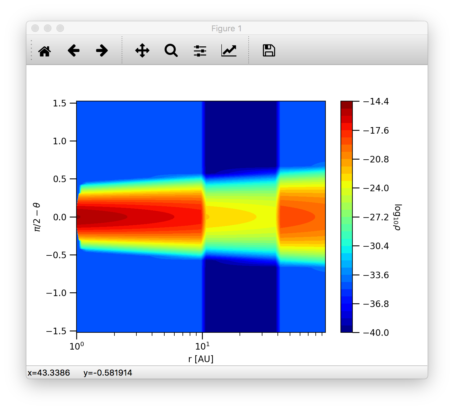
Dust density contours
radmc3dData stores not only the physical variables as data attributes, but also the wavelength and spatial grids
(radmc3dData.grid attribute, which is an instance of the radmc3dGrid class).
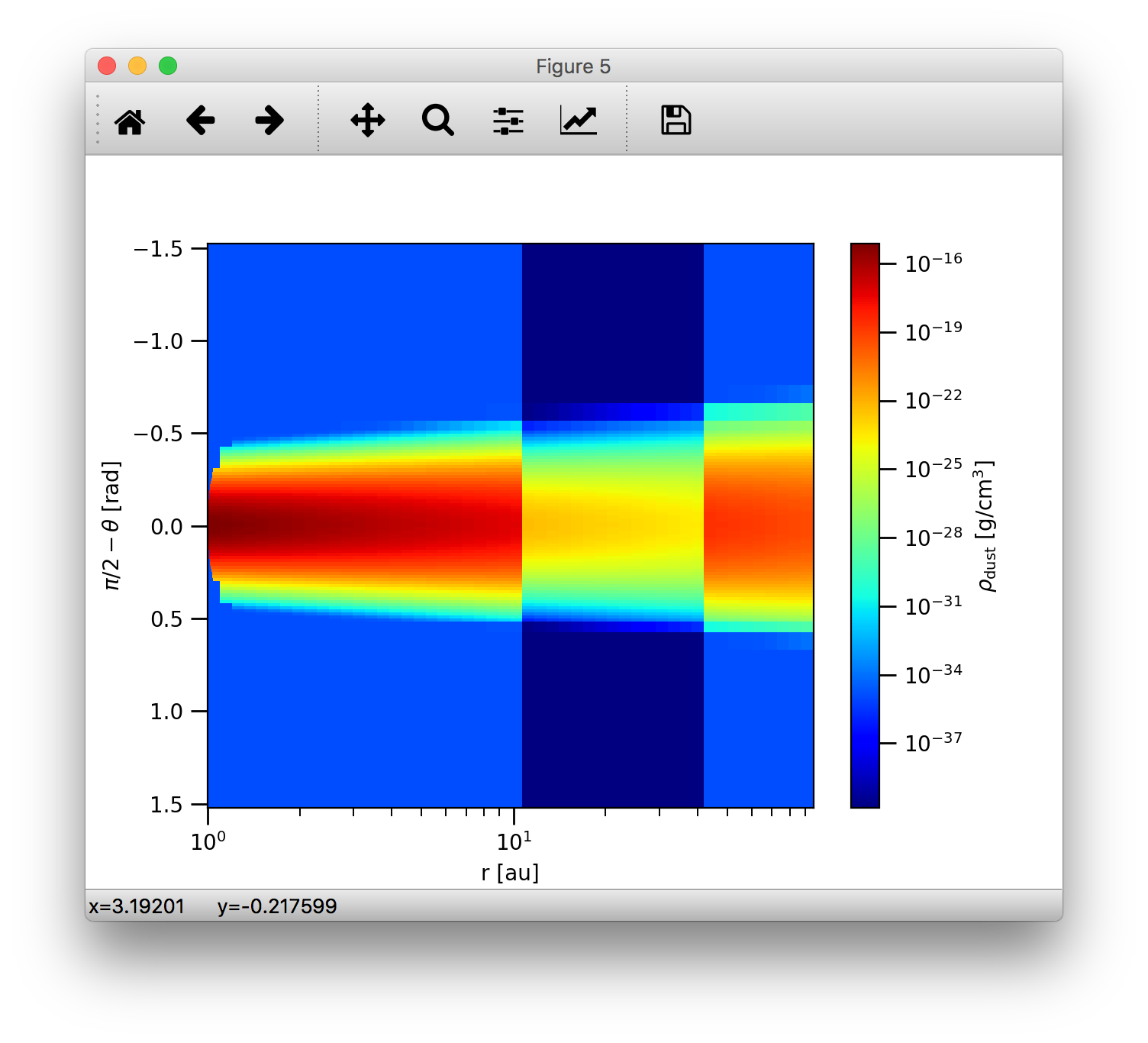
So we can make 2D density contour plot.
>>> c = plb.contourf(data.grid.x/natconst.au, np.pi/2.-data.grid.y, np.log10(data.rhodust[:,:,0,0].T), 30)
>>> plb.xlabel('r [AU]')
>>> plb.ylabel(r'$\pi/2-\theta$')
>>> plb.xscale('log')
Adding colorbars in matplotlib is really easy:
>>> cb = plb.colorbar(c)
>>> cb.set_label(r'$\log_{10}{\rho}$', rotation=270.)
The end result should look like this:
Dust opacity
The readOpac() function in the analyze module can be used to read the dust opacity.
One can either pass the extension tag name of the dust opacity file (dustkappa_NAME.inp). We can read e.g. the dustkappa_silicate.inp
as:
>>> opac = analyze.readOpac(ext=['silicate'])
alternatively one can also pass the index of the dust component in the dust density array. The command to read the first dust species in the dust density distribution:
>>> opac = analyze.readOpac(idust=[0])
Note, that python also starts the array/list indices from zero, hence the first dust species in the dust density array will have the index of zero.
The readOpac() function returns an instance of the radmc3dDustOpac class.
The data attributes of this class are all lists, containing the opacity data of an individual dust component.
We can plot the absorption coefficient as a function of wavelength as:
>>> plb.loglog(opac.wav[0], opac.kabs[0])
>>> plb.xlabel(r'$\lambda$ [$\mu$m]')
>>> plb.ylabel(r'$\kappa_{\rm abs}$ [cm$^2$/g]')
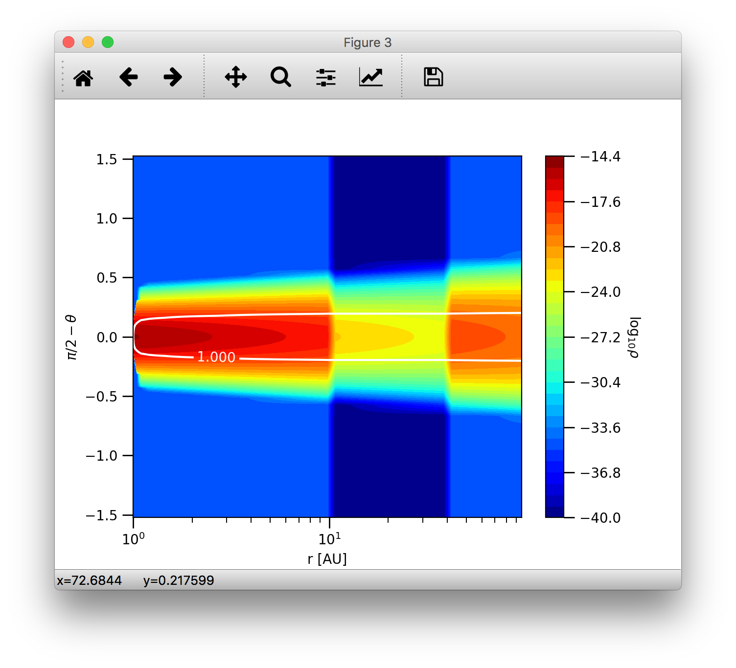
As mentioned, the 0-index of the wav and kabs attributes means that we want to plot the wavelength and absorption coefficient
of the first dust species, that has actually been read. The indices in the data attributes mean only the sequential order as
the data have been read. The index of this dust species in the dust density array is given by radmc3dDustOpac.idust, which is also
a list.
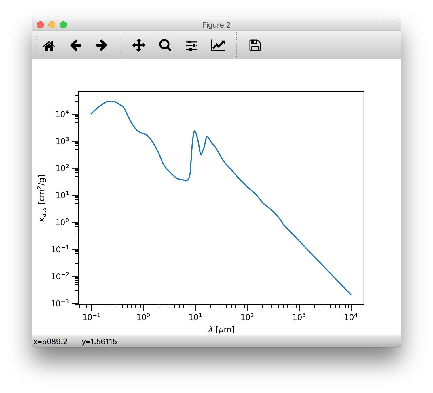
Optical depth
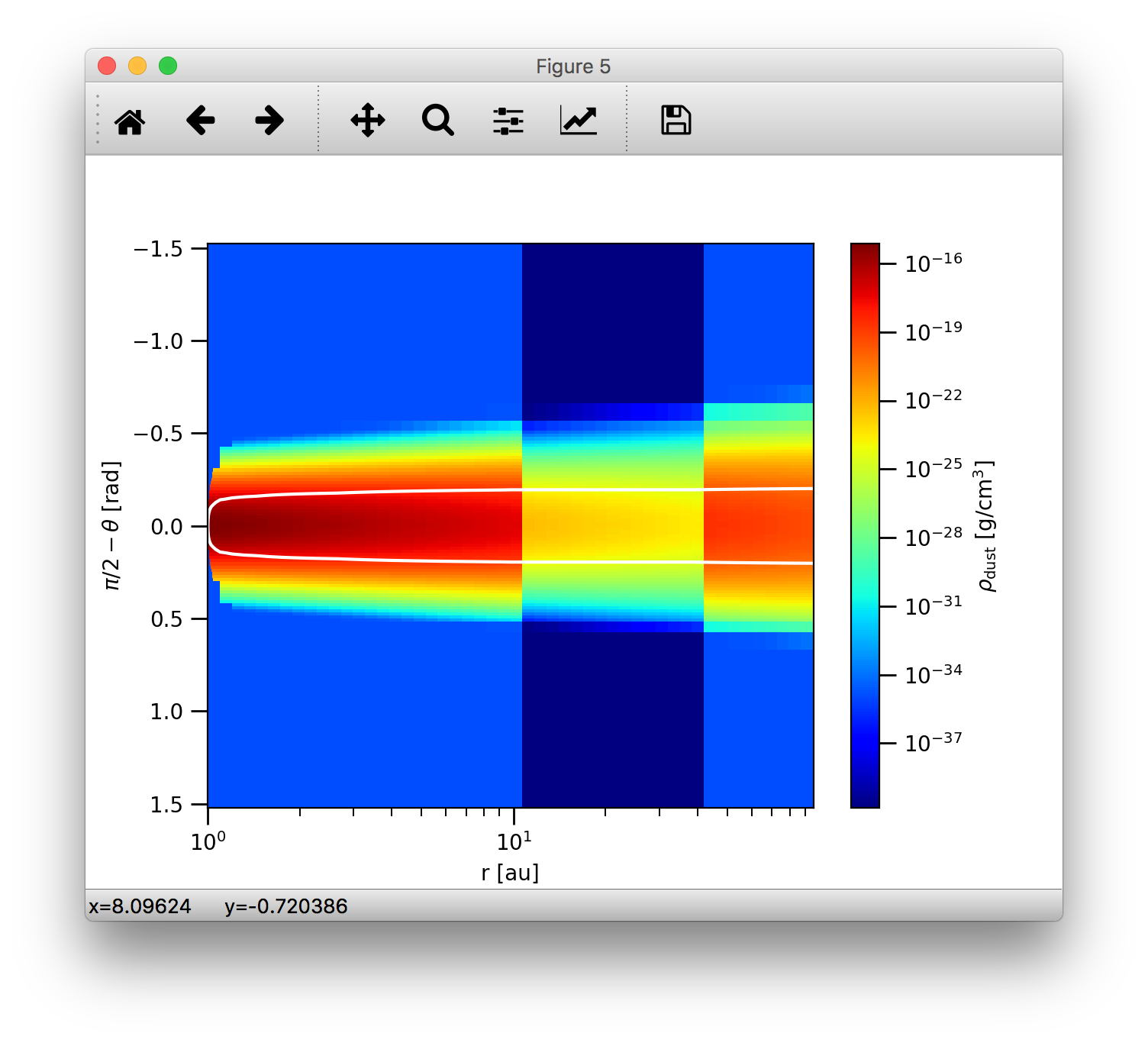
It is useful to display where the radial optical depth in the continuum at the peak of the stellar radiation field is located.
The getTau() method of the radmc3dData class calculates the
optical depth.:
>>> data.getTau(wav=0.5)
 Opacity at 0.50um :  19625.9938111
The getTau() method puts the optical depth into the radmc3dData.tauy and
radmc3dData.tauy attributes. So we can now also overplot the radial optical depth of unity contour:
>>> c = plb.contour(data.grid.x/natconst.au, np.pi/2.-data.grid.y, data.taux[:,:,0].T, [1.0],  colors='w', linestyles='solid')
>>> plb.clabel(c, inline=1, fontsize=10)
Run the thermal MC
To calculate the temperature distribution in the disk we need to run RADMC-3D in thermal Monte Carlo mode. This can be done from within the python shell:
>>> import os
>>> os.system('radmc3d mctherm')
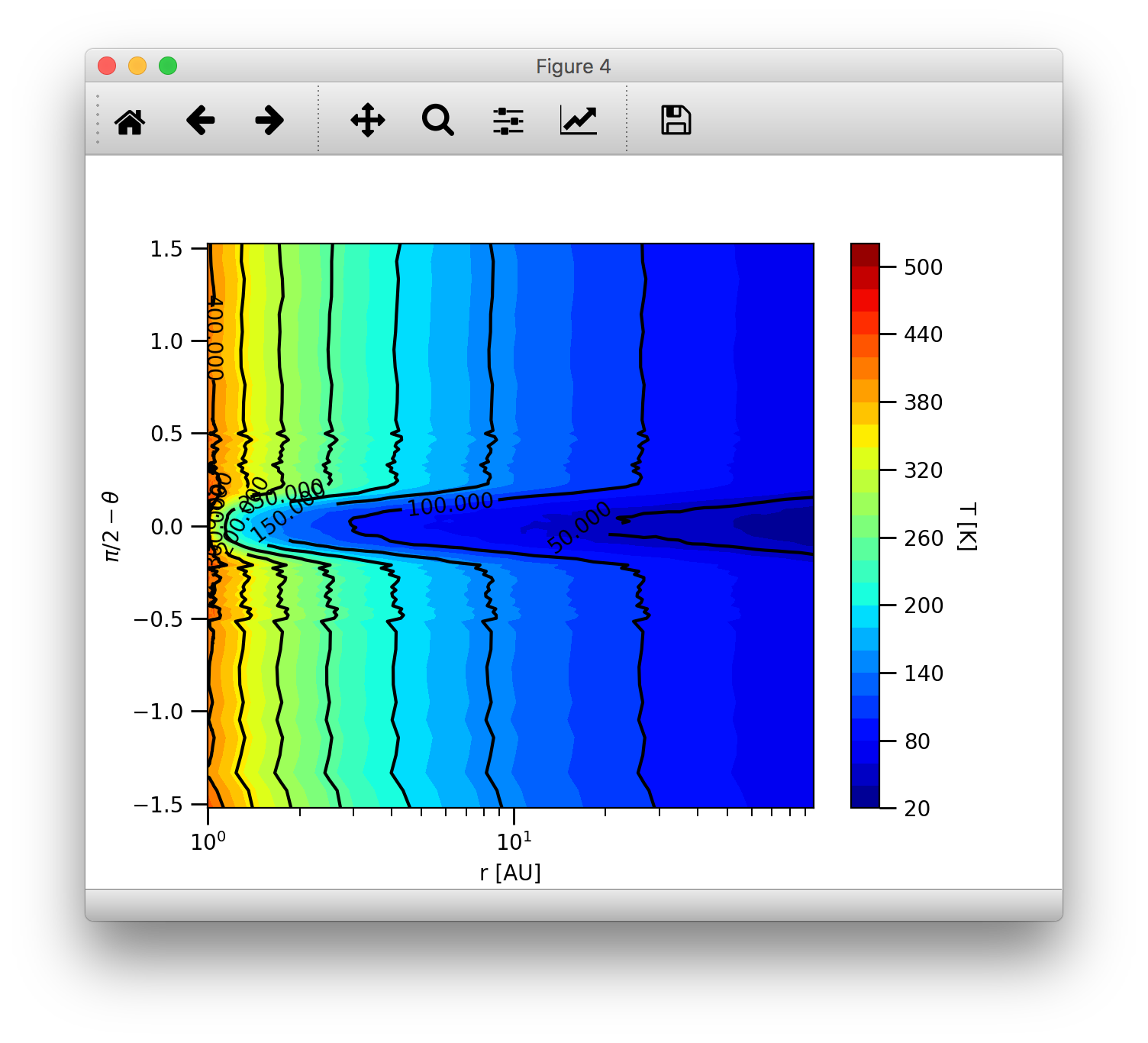
Dust temperature contours
After the thermal Monte Carlo simulation has successfully finished we can read the calculated dust temperature:
>>> data = analyze.readData(dtemp=True)
Reading dust temperature
Alternatively we can also use the previous instance of the radmc3dData we used to get the dust density,
to read the dust temperature. The readData() function is only an interface to the methods of the
radmc3dData class.:
>>> data = analyze.readData(dtemp=True)
Reading dust density
>>> data.readDustTemp()
Reading dust temperature
Then we can plot the 2D temperature contours:
>>> c = plb.contourf(data.grid.x/natconst.au, np.pi/2.-data.grid.y, data.dusttemp[:,:,0,0].T, 30)
>>> plb.xlabel('r [AU]')
>>> plb.ylabel(r'$\pi/2-\theta$')
>>> plb.xscale('log')
>>> cb = plb.colorbar(c)
>>> cb.set_label('T [K]', rotation=270.)

>>> c = plb.contour(data.grid.x/natconst.au, np.pi/2.-data.grid.y, data.dusttemp[:,:,0,0].T, 10,  colors='k', linestyles='solid')
>>> plb.clabel(c, inline=1, fontsize=10)
Then the result should look like this:
Convenient 2D contour plots
From version v0.29 there is a new convenient way to do 2D contour plots using the function plotSlice2D().
It can be used to make 2D slice plots (both contours and colorscale maps) with a single command. E.g. the dust density in a vertical slice
can be plotted with the command:
>>>analyze.plotSlice2D(data, var='ddens', plane='xy', log=True, linunit='au', cmap=plb.cm.jet)
>>>plb.xscale('log')
which should result in the following plot
Note, that the difference between the colorscale maps produced by plotSlice2D() and the contour plot made above is that
while previously we used a the countourf function of matplotlib to produce a filled contour plot plotSlice2D() uses
the pcolormesh function to display the colorscale map. We can also overlay contour lines to display e.g. the optical depth:
>>>data.getTau(wav=0.5)
>>>analyze.plotSlice2D(data, var='taux', plane='xy', log=True, linunit='au', contours=True, clev=[1.0], clcol='w')
This should add a white contour line of the previously generated colorscale map
We can also add another layer of contour line overlay by displaying dust temperature contours. Let us show the contour of the 150K region:
>>>analyze.plotSlice2D(data, var='dtemp', plane='xy', ispec=0, log=True, linunit='au', contours=True, clev=[150.0], clcol='k', cllabel=True)
Note, that for dust temperature plots one should always set the dust species index using the ispec keyword. The clev keyword controls
the value of the contour line(s), clcol sets the contour line color and cllabel sets whether or not the values of the contour lines should
also be displayed. The resulting plot should look like this

Images
Make an image
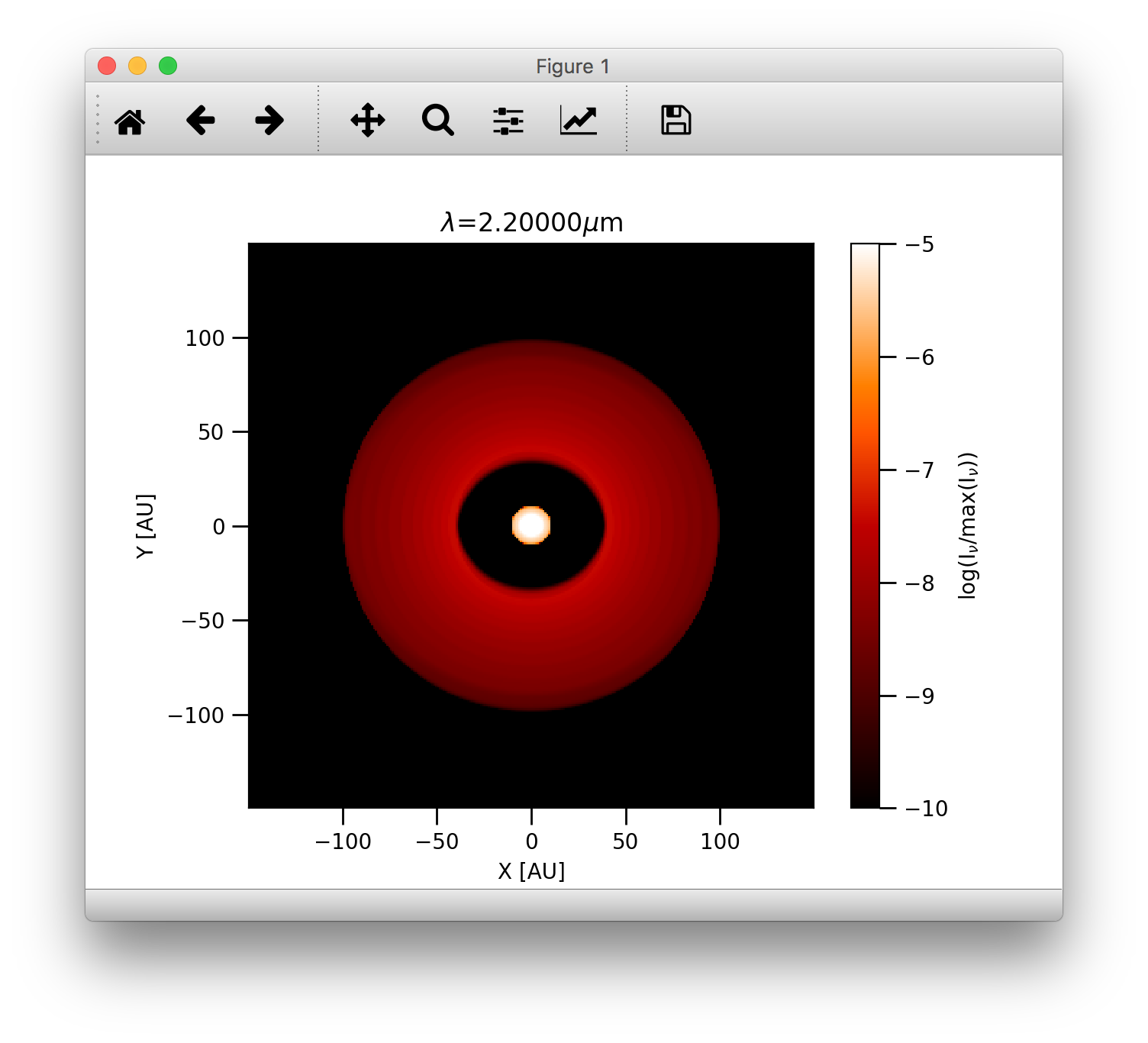
Images can be calculated using the makeImage() method
>>> image.makeImage(npix=300., wav=2.2, incl=20., phi=0., sizeau=300.)

 ================================================================
      WELCOME TO RADMC-3D: A 3-D CONTINUUM AND LINE RT SOLVER

        This is the 3-D reincarnation of the 2-D RADMC code
                (c) 2010/2011 Cornelis Dullemond

 ************* NOTE: THIS IS STILL A BETA VERSION ***************
 ****** Some modes/capabilities are not yet ready/mature ********

       Please feel free to ask questions. Also please report
        bugs and/or suspicious behavior without hestitation.
      The reliability of this code depends on your vigilance!

   To keep up-to-date with bug-alarms and bugfixes, register to
      the RADMC-3D mailing list by sending an email to me:
        dullemon@mpia.de or dullemond@uni-heidelberg.de

              Please visit the RADMC-3D home page at
  http://www.ita.uni-heidelberg.de/~dullemond/software/radmc-3d/
 ================================================================

 Note: T_gas taken to be equal to T_dust of dust species            1
 Reading global frequencies/wavelengths...
 Reading grid file and prepare grid tree...
    Adjusting theta(ny+1) to exactly pi...
    Adjusting theta(41) to exactly pi/2...
 Reading star data...
 Note: Please be aware that you treat the star(s) as
       point source(s) while using spherical coordinate mode.
       Since R_*<<R_in this is probably OK, but if you want
       to play safe, then set istar_sphere = 1 in radmc3d.inp.
 Note: Star 1 is taken to be a blackbody star
       at a temperature T = 4000. Kelvin
 Grid information (current status):
   We have 6800 branches, of which 6800 are actual grid cells.
   ---> 100.000% mem use for branches, and 100.000% mem use for actual cells.
   No grid refinement is active. The AMR tree is not allocated (this saves memory).
 ALWAYS SELF-CHECK FOR NOW...
 Starting procedure for rendering image...
   --> Including dust
       No lines included...
       No gas continuum included...
 Reading dust data...
 Note: Opacity file dustkappa_silicate.inp does not cover the
       complete wavelength range of the model (i.e. the range
       in the file frequency.inp or wavelength_micron.inp).
       Range of model:     lambda = [ 0.10E+00, 0.10E+05]
       Range in this file: lambda = [ 0.10E+00, 0.10E+05]
       Simple extrapolations are used to extend this range.
 Reading dust densities...
 Dust mass total =    6.9721299190506066E-008  Msun
 Reading dust temperatures...
 Rendering image(s)...
 Doing scattering Monte Carlo simulation for lambda =    2.2000000000000002       micron...
 Using dust scattering mode            1
 Wavelength nr            1  corresponding to lambda=   2.2000000000000002       micron
    Photon nr         1000
    .
    .
    .
    Photon nr        30000
 Average number of scattering events per photon package =    5.9100000000000000E-002
 Ray-tracing image for lambda =    2.2000000000000002       micron...
 Writing image to file...
 Used scattering_mode=1, meaning: isotropic scattering approximation.
 Diagnostics of flux-conservation (sub-pixeling):
     Nr of main pixels (nx*ny)   =        90000
     Nr of (sub)pixels raytraced =       204616
     Nr of (sub)pixels used      =       175962
     Increase of raytracing cost =    2.2735111111111110
 Done...
Display images
Now we can read the image:
>>> im = image.readImage()
To display the images calculated by RADMC-3D we can use the plotImage() method
>>> image.plotImage(im, au=True, log=True, maxlog=10, saturate=1e-5, cmap=plb.cm.gist_heat)
The results should look like this:
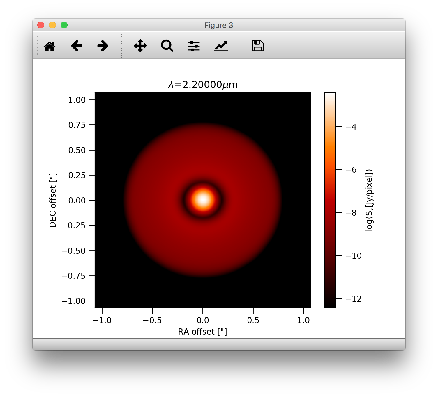
We can also display the images using angular coordinates for the image axis (Note that in this case the distance in pc needs also to be passed):
>>> image.plotImage(im, arcsec=True, dpc=140., log=True, maxlog=10, saturate=1e-5, bunit='snu', cmap=plb.cm.gist_heat)
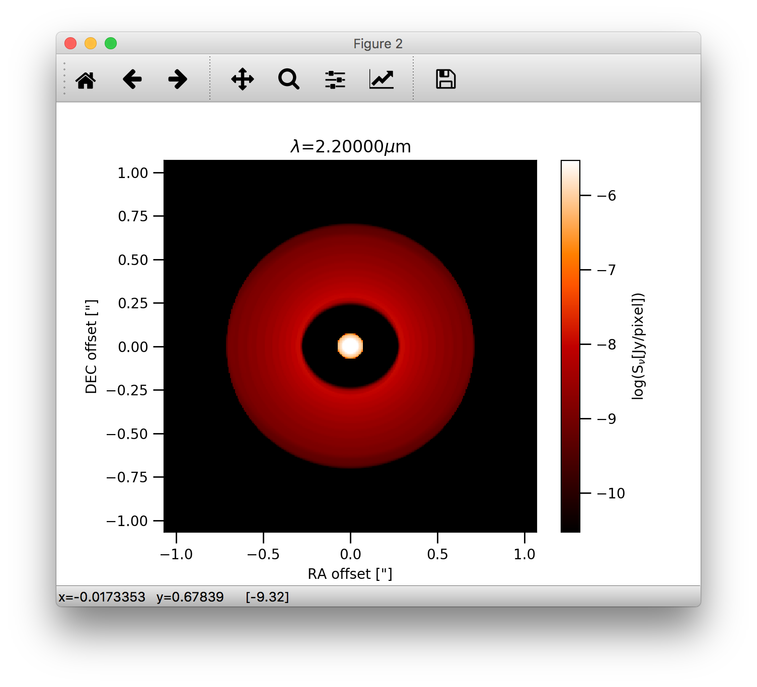
Image manipulations
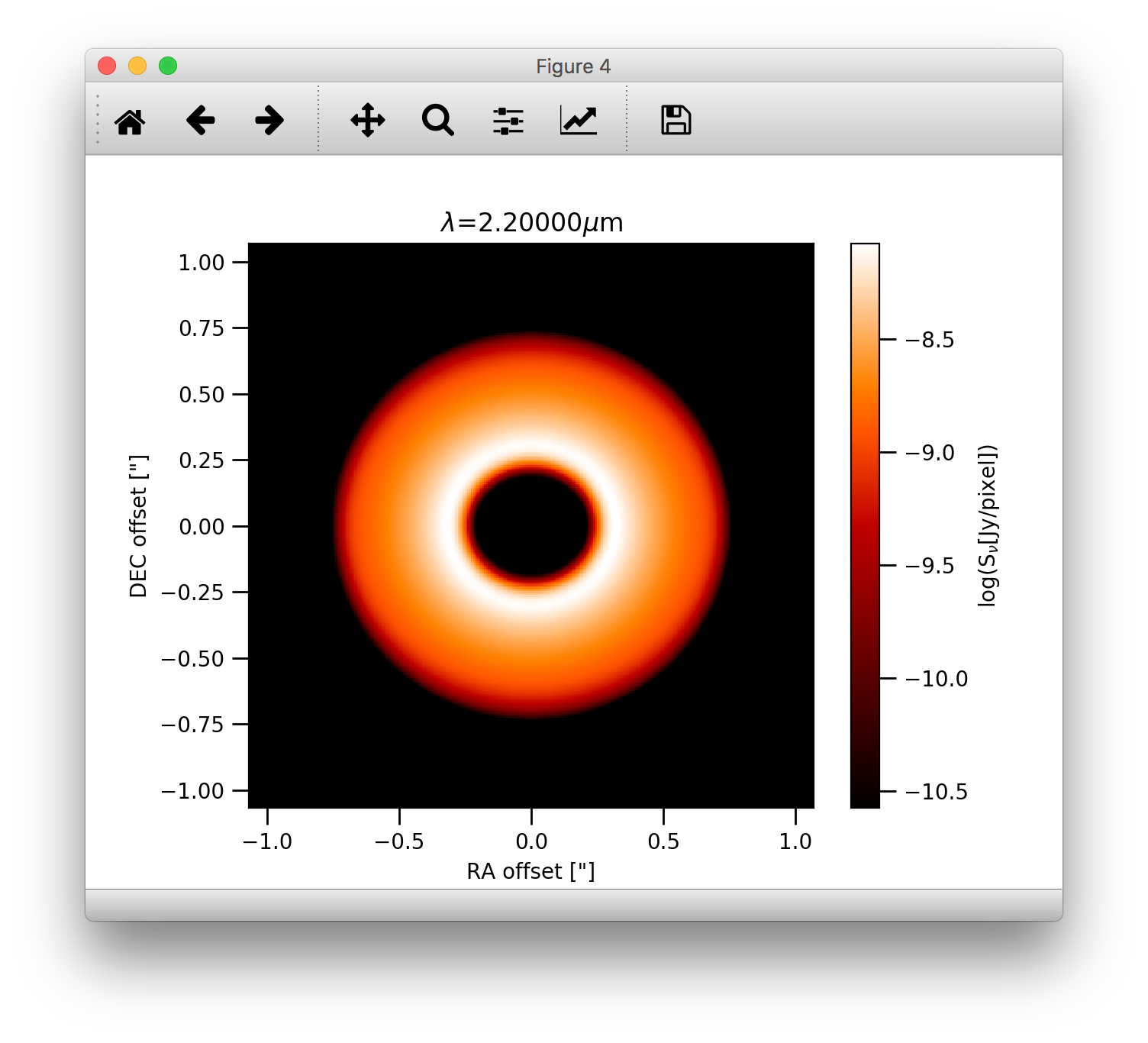
It is also easy to convolve the image with an arbitrary 2D gaussian beam:
>>> cim = im.imConv(fwhm=[0.06, 0.06], pa=0., dpc=140.)
>>> image.plotImage(cim, arcsec=True, dpc=140., log=True, maxlog=10, bunit='snu', cmap=plb.cm.gist_heat)
The effect of a coronographic mask can also be simulated. The cmask_rad keyword of the plotImage() method sets the
intensity within the given radius to zero.:
>>> image.plotImage(cim, arcsec=True, dpc=140., log=True, maxlog=2.5, bunit='snu', cmask_rad=0.17, cmap=plb.cm.gist_heat)
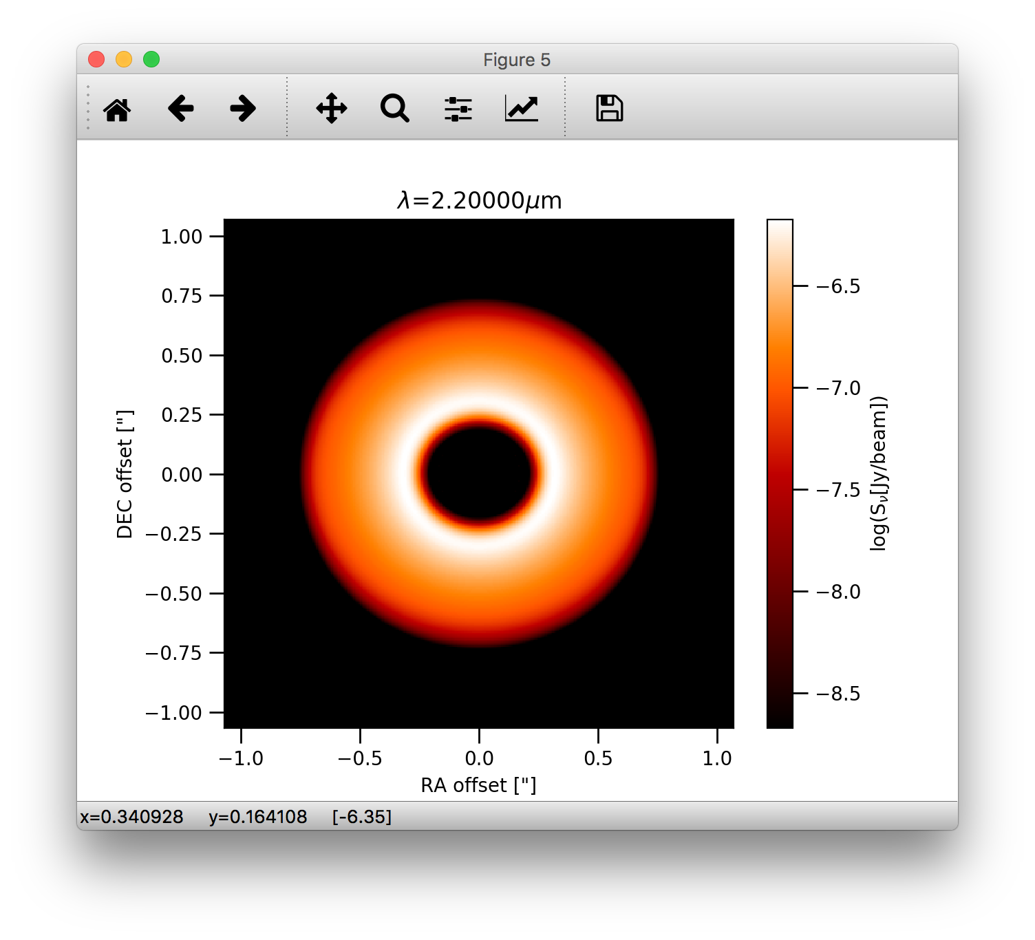
Note, that one can also use the bunit='jy/pixel keyword to display the image in units of Jy/pixel. The bunit='snu' is kept
for backward compatibility for now. To display the image in units of Jy/beam for the intensity we can use the bunit='jy/beam' keyword:
>>> image.plotImage(cim, arcsec=True, dpc=140., log=True, maxlog=2.5, bunit='jy/beam', cmask_rad=0.17, cmap=plb.cm.gist_heat)
which should produce the following image:
Writing images to fits
We can also write the image to a fits file with the writeFits() method:
im.writeFits('myimage.fits', dpc=140., coord='03h10m05s -10d05m30s')
It takes at very least two arguments, the name of the file and the distance in parsec.