Dust continuum radiative transfer
Many of the things related to dust continuum radiative transfer have already been said in the previous chapters. But here we combine these things, and expand with more in-depth information.
Most users simply want RADMC-3D to compute images and spectra from a model. This is done in a two-stage procedure:
First compute the dust temperature everywhere using the thermal Monte Carlo computation (Section The thermal Monte Carlo simulation: computing the dust temperature).
Then making the images and/or spectra (Section Making SEDs, spectra, images for dust continuum).
You can then view the output spectra and images with the Python tools or use your own plotting software.
Some expert users may wish to use RADMC-3D for something entirely different: to compute the local radiation field {em inside} a model, and use this for e.g. computing photochemistry rates of a chemical model or so. This is described in Section Special-purpose feature: Computing the local radiation field.
You may also use the thermal Monte Carlo computation of the dust temperature to help estimating the {em gas} temperature for the line radiative transfer. See Chapter Line radiative transfer for more on line transfer.
The thermal Monte Carlo simulation: computing the dust temperature
RADMC-3D can compute the dust temperature using the Monte Carlo method of
Bjorkman & Wood (2001, ApJ 554, 615) with various improvements such as the
continuous absorption method of Lucy (1999, A&A 344, 282). Once a model is
entirely set up, you can ask radmc3d to do the Monte Carlo
run for you by typing in a shell:
radmc3d mctherm
if you use the standard radmc3d code, or
./radmc3d mctherm
if you have created a local version of radmc3d (see Section
Making special-purpose modified versions of RADMC-3D (optional)).
What the method does is the following: First all the netto sources of energy (or more accurately: sources of luminosity) are identified. The following net sources of energy can be included:
Stars: You can specify any number of individual stars: their position, and their spectrum and luminosity (See Section INPUT (mostly required): stars.inp). This is the most commonly used source of luminosity, and as a beginning user we recommend to use only this for now.
Continuum stellar source: For simulations of galaxies it would require by far too many individual stars to properly include the input of stellar light from the billions of stars in the galaxy. To overcome this problem you can specify a continuously spatially distributed source of stars. NOTE: Still in testing phase.
Viscous heating / internal heating: Sometimes the dust grains acquire energy directly from the gas, for instance through viscous heating of the gas or adiabatic compression of the gas. This can be included as a spatially distributed source of energy. NOTE: Still in progress… Not yet working.
To compute the dust temperature we must have at least one source of luminosity, otherwise the equilibrium dust temperature would be everywhere 0.
The next step is that this total luminosity is divided into nphot packages,
where nphot is 100000 by default, but can be set to any value by the user
(see the file radmc3d.inp described in Section INPUT: radmc3d.inp). Then
these photon packages are emitted by these sources one-by-one. As they move
through the grid they may scatter off dust grains and thus change their
direction. They may also get absorbed by the dust. If that happens, the photon
package is immediately re-emitted in another direction and with another
wavelength. The wavelength is chosen according to the recipe by Bjorkman & Wood
(2001, ApJ 554, 615). The luminosity fraction that each photon package
represents remains, however, the same. Each time a photon package enters a cell
it increases the ‘energy’ of this cell and thus increases the temperature of
the dust of this cell. The recipe for this is again described by Bjorkman &
Wood (2001, ApJ 554, 615), but contrary to that paper we increase the
temperature of the dust always when a photon package enters a cell, while
Bjorkman & Wood only increase the dust temperature if a discrete absorption
event has taken place. Each photon package will ping-pong through the model and
never gets lost until it escapes the model through the outer edge of the grid
(which, for cartesianl coordinates, is any of the grid edges in \(x\),
\(y\) or \(z\), and for spherical coordinates is the outer edge of
\(r\)). Once it escapes, a new photon package is launched, until also it
escapes. After all photon packages have been launched and escaped, the dust
temperature that remains is the final answer of the dust temperature.
One must keep in mind that the temperature thus computed is an equilibrium dust temperature. It assumes that each dust grain acquires as much energy as it radiates away. This is for most cases presumably a very good approximation, because the heating/cooling time scales for dust grains are typically very short compared to any time-dependent dynamics of the system. But there might be situations where this may not be true: in case of rapid compression of gas, near shock waves or in extremely optically thick regions.
NOTE: Monte Carlo simulations are based on pseudo-random numbers. The seed for the random number generator is by default set to -17933201. If you want to perform multiple identical simulations with a different random sequence you will need to set the seed by hand. This can be done by adding a line
iseed = -5415
(where -5415 is to be replaced by the value you want) to the radmc3d.inp file.
Modified Random Walk method for high optical depths
As you will soon find out: very optically thick models make the RADMC-3D thermal Monte Carlo simulations to be slow. This is because in the thermal Monte Carlo method a photon package is never destroyed unless it leaves the system. A photon package can thus ‘get lost’ deep inside an optically thick region, making millions (or even billions) of absorption+reemission or scattering events. Furthermore, you will notice that in order to get the temperatures in these very optically thick regions to be reliable (i.e. not too noisy) you may need a very large number of photon packages for your simulation, which slows down the simulation even more. It is hard to prevent such problems. Min, Dullemond, Dominik, de Koter & Hovenier (2009) A&A 497, 155 discuss two methods of dealing with this problem. One is a diffusion method, which we will not discuss here. The other is the ‘Modified Random Walk’ (MRW) method, based on the method by Fleck & Canfield (1984) J.Comput.Phys. 54, 508. Note that Robitaille (2010) A&A 520, 70 presented a simplification of this method. Min et al. first implemented this method into the MCMax code. It is also implemented in RADMC-3D, in Robitaille’s simplified form.
The crucial idea of the method is that if a photon package ‘gets lost’ deep inside a single ultra-optically-thick cell, we can use the analytical solutions of the diffusion equation in a constant-density medium to predict where the photon package will go next. This thus allows RADMC-3D to make a single large step of the photon package which actually corresponds to hundreds or thousands of absorption+reemission or scattering events.
The method works best if the optically thick cells are as large as possible. This is because the analytical solutions are only valid within a single cell, and thus the ‘large step’ can not be larger than a single cell size. Moreover, cell crossings will reduce the step length again to the physical mean free path, so the more cell crossings are made, the less effective the MRW becomes.
NOTE: The MRW is by default switched off. The reason is that it is, after all, an approximation. However, if RADMC-3D thinks that the MRW may help speed up the thermal Monte Carlo, it will make the suggestion to the user to switch on the MRW method.
NOTE: So far the MRW method is only implemented using the Planck mean opacity for estimating the ‘large step’. This could, under certain conditions, be inaccurate. The reason why the (more accurate) Rosseland mean opacity is not used is that this precludes the precomputation and tabulation of the mean opacities if multiple independent dust species are used. Strictly speaking, even the Rosseland mean opacity is not entirely correct, but it is a good approximation (see Min et al. 2009). So far these simplifications do not seem to matter a lot. But if strong effects are seen, please report these. Conditions under which it is likely to make a difference (i.e. the present implementation becoming inaccurate) are when an internal heat source inside a super-optically thick region is introduced (e.g. viscous heating in a disk), and/or when the opacities are extremely wavelength-dependent (varying by orders of magnitude in small distances in wavelengths). So please use MRW with care. Upon request we may implement the true MRW: with the Rosseland mean, which, however, may make the code slower.
You can switch on the MRW by adding the following line to the
radmc3d.inp file:
modified_random_walk = 1
Making SEDs, spectra, images for dust continuum
You can use RADMC-3D for computing spectra and images in dust continuum
emission. This is described in detail in Chapter
Making images and spectra. RADMC-3D needs to know not only the dust spatial
distribution, given in the file dust_density.inp, but also the
dust temperature, given in the file dust_temperature.dat (see
Chapter Binary I/O files for the binary version of these files, which
are more compact, and which you can use instead of the ascii versions). The
dust_temperature.dat is normally computed by RADMC-3D itself
through the thermal Monte Carlo computation (see Section
The thermal Monte Carlo simulation: computing the dust temperature). But if you, the user, wants to specify
the dust temperature at each location in the model youself, then you can
simply create your own file dust_temperature.dat and skip the
thermal Monte Carlo simulation and go straight to the creation of images or
spectra.
The basic command to make a spectrum at the global grid of wavelength
(specified in the file wavelength_micron.inp,
see Section INPUT (required): wavelength_micron.inp) is:
radmc3d sed
You can specify the direction of the observer with incl and phi:
radmc3d sed incl 20 phi 80
which means: put the observer at inclination 20 degrees and \(\phi\)-angle 80 degrees.
You can also make a spectrum for a given grid of wavelength (independent of the
global wavelength grid). You first create a file
camera_wavelength_micron.inp, which has the same format as
wavelength_micron.inp. You can put any set of wavelengths in this file
without modifying the global wavelength grid (which is used by the thermal Monte
Carlo computation). Then you type
radmc3d spectrum loadlambda
and it will create the spectrum on this wavelength grid. More information about making spectra is given in Chapter Making images and spectra.
For creating an image you can type
radmc3d image lambda 10
which creates an image at wavelength \(\lambda`=10:math:\)mu`m. More information about making images is given in Chapter Making images and spectra.
Important note: To handle scattering of light off dust grains, the ray-tracing is preceded by a quick Monte Carlo run that is specially designed to compute the ‘scattering source function’. This Monte Carlo run is usually much faster than the thermal Monte Carlo run, but must be done at each wavelength. It can lead, however, to slight spectral noise, because the random photon paths are different for each wavelength. See Section More about scattering of photons off dust grains for details.
OpenMP parallelized Monte Carlo
Depending on the model properties and the number of photon packages used in the simulation the Monte Carlo calculation (in particular the thermal Monte Carlo, but under some conditions also the scattering Monte Carlo) can be a time-consuming computation when executed only in a serial mode. To improve this, these Monte Carlo calculations can be done in OpenMP parallel mode. The loop over photon packages is then distributed amongst the different threads, where each thread adopts a specific number of loop iterations following the order of the thread identification number. To this end the random number generator was modified. The important point for the parallel version is that different threads must not share the same random seed initially. To be certain that each thread is assigned a different seed at the beginning, the thread identity number is added to the initial seed.
The default value for the number of threads in the parallel version is set to
one, so that the program is identical with the serial version, except for the
random generator’s initial seed. The user can change the value by either typing
setthreads <nr>, where <nr> is the number of requested threads (integer
value) in the command line or by adding a corresponding line to the
radmc3d.inp file. If the chosen number of threads is larger than the
available number of processor cores, the user is asked to reduce it.
For example, you can ask radmc3d to do the parallelized Monte
Carlo run for you by typing in a shell:
radmc3d mctherm setthreads 4
or by adding the following keyword to the radmc3d.inp file:
setthreads = 4
which means that four threads are used for the thermal Monte Carlo computation.
For the image or spectrum you can do the same: just add setthreads 4 or so
on the command line or put setthreads = 4 into the radmc3d.inp file.
Make sure that you have included the -fopenmp keyword in the Makefile
and have compiled the whole radmc3d source code with this additional command
before using the OpenMP parallelized thermal Monte Carlo version (cf. Section
Compiling the code with ‘make’).
Overview of input data for dust radiative transfer
In order to perform any of the actions described in Sections The thermal Monte Carlo simulation: computing the dust temperature, Special-purpose feature: Computing the local radiation field or Making SEDs, spectra, images for dust continuum, you must give RADMC-3D the following data:
amr_grid.inp: The grid file (see Section INPUT (required): amr_grid.inp).wavelength_micron.inp: The global wavelength file (see Section INPUT (required): wavelength_micron.inp).stars.inp: The locations and properties of stars (see Section INPUT (mostly required): stars.inp).dust_density.inp: The spatial distribution of dust on the grid (see Section INPUT (required for dust transfer): dust_density.inp).dustopac.inp: A file with overall information about the various species of dust in the model (see Section INPUT (required for dust transfer): dustopac.inp and dustkappa_*.inp or dustkapscatmat_*.inp or dust_optnk_*.inp). One of the main pieces of information here is (a) how many dust species are included in the model and (b) the tag names of these dust species (seedustkappa_XXX.inpbelow). The filedust_density.inpmust contain exactly this number of density distributions: one density distribution for each dust species.dustkappa_XXX.inp: One or more dust opacity files (whereXXXshould in fact be a tag name you define, for instancedustkappa_silicate.inp). The labels are listed in thedustopac.inpfile. See Section INPUT (required for dust transfer): dustopac.inp and dustkappa_*.inp or dustkapscatmat_*.inp or dust_optnk_*.inp for more information.camera_wavelength_micron.inp (optional): This file is only needed if you want to create a spectrum at a special set of wavelengths (otherwise useradmc3d sed).mcmono_wavelength_micron.inp (optional): This file is only needed if you want to compute the radiation field inside the model by callingradmc3d mcmono(e.g. for photochemistry).
Other input files could be required in certain cases, but you will then be asked about it by RADMC-3D.
Special-purpose feature: Computing the local radiation field
If you wish to use RADMC-3D for computing the radiation field inside the model, for instance for computing photochemical rates in a chemical model, then RADMC-3D can do so by calling RADMC-3D in the following way:
radmc3d
mcmono
This computes the mean intensity
(in units of
\(\mathrm{erg}\,\mathrm{s}^{-1}\,\mathrm{cm}^{-2}\,\mathrm{Hz}^{-1}\,\mathrm{ster}^{-1}\))
as a function of the \((x,y,z)\) (cartesian) or \((r,\theta,\phi)\)
(spherical) coordinates at frequencies \(\nu_i\equiv 10^4c/\lambda_i\) where
\(\lambda_i\) are the wavelengths (in \(\mu\)m) specified in the file mcmono_wavelength_micron.inp (same format as the file
wavelength_micron.inp which is described in Section
INPUT (required): wavelength_micron.inp). The results of this computation can be interesting for,
for instance, models of photochemistry.
The file that is produced by radmc3d mcmono is called
mean_intensity.out and has the following form:
iformat                                  <=== Typically 2 at present
nrcells
nfreq                                    <=== Nr of frequencies
freq_1 freq_2 ... freq_nfreq             <=== List of frequencies in Hz
meanint[1,icell=1]
meanint[1,icell=2]
...
meanint[1,icell=nrcells]
meanint[2,icell=1]
meanint[2,icell=2]
...
meanint[2,icell=nrcells]
...
...
...
meanint[nfreq,icell=1]
meanint[nfreq,icell=2]
...
meanint[nfreq,icell=nrcells]
The list of frequencies will, in fact, be the same as those listed in the file
mcmono_wavelength_micron.inp.
Note that if your model is very large, the computation of the radiation field on a large set of wavelength could easily overload the memory of the computer. However, often you are in the end not interested in the entire spectrum at each location, but just in integrals of this spectrum over some cross section. For instance, if you want to compute the degree to which dust shields molecular photodissociation lines in the UV, then you only need to compute the total photodissociation rate, which is an integral of the photodissociation cross section times the radiation field. In Section Using the userdef module to compute integrals of J_\nu it will be explained how you can create a userdef subroutine (see Chapter Modifying RADMC-3D: Internal setup and user-specified radiative processes) that will do this for you in a memory-saving way.
There is an important parameter for this Monochromatic Monte Carlo that you may wish to play with:
nphot_monoThe parameternphot_monosets the number of photon packages that are used for the Monochromatic Monte Carlo simulation. It has as default 100000, but that may be too little for 3-D models. You can set this value in two ways:In the
radmc3d.inpfile as a linenphot_mono = 1000000for instance.On the command-line by adding
nphot_mono 1000000.
More about scattering of photons off dust grains
Photons can not only be absorbed and re-emitted by dust grains: They can also be scattered. Scattering does nothing else than change the direction of propagation of a photon, and in case polarization is included, its Stokes parameters. Strictly speaking it may also slightly change its wavelength, if the dust grains move with considerable speed they may Doppler-shift the wavelength of the outgoing photon (which may be relevant, if at all, when dust radiative transfer is combined with line radiative transfer, see chapter Line radiative transfer), but this subtle effect is not treated in RADMC-3D. For RADMC-3D scattering is just the changing of direction of a photon.
Five modes of treating scattering
RADMC-3D has five levels of realism of treatment of scattering, starting
with scattering_mode=1 (simplest) to scattering_mode=5 (most realistic):
No scattering (
scattering_mode=0):If either the
dustkappa_XXX.inpfiles do not contain a scattering opacity or scattering is switched off by settingscattering_mode_maxto 0 in theradmc3d.inpfile, then scattering is ignored. It is then assumed that the dust grains have zero albedo.Isotropic scattering (
scattering_mode=1):If either the
dustkappa_XXX.inpfiles do not contain information about the anisotropy of the scattering or anisotropic scattering is switched off by settingscattering_mode_maxto 1 in theradmc3d.inpfile, then scattering is treated as isotropic scattering. Note that this can be a bad approximation.Anisotropic scattering using Henyey-Greenstein (
scattering_mode=2):If the
dustkappa_XXX.inpfiles contain the scattering opacity and the \(g\) parameter of anisotropy (the Henyey-Greenstein \(g\) parameter which is equal, by definition, to \(g=\langle\cos\theta\rangle\), where \(\theta\) is the scattering deflection angle), andscattering_mode_maxis set to 2 or higher in theradmc3d.inpfile then anisotropic scattering is treated using the Henyey-Greenstein approximate formula.Anisotropic scattering using tabulated phase function (
scattering_mode=3):To treat scattering using a tabulated phase function, you must specify the dust opacities using
dustkapscatmat_XXX.inpfiles instead of the simplerdustkappa_XXX.inpfiles (see Section The dustkapscatmat_*.inp files). You must also setscattering_mode_maxis set to 3 or higher.Anisotropic scattering with polarization for last scattering (
scattering_mode=4):To treat scattering off randomly oriented particles with the full polarization you need to set
scattering_mode_maxis set to 4 or higher, and you must specify the full dust opacity and scattering matrix using thedustkapscatmat_XXX.inpfiles instead of the simplerdustkappa_XXX.inpfiles (see Section The dustkapscatmat_*.inp files). Ifscattering_mode=4the full polarization is only done upon the last scattering before light reaches the observer (i.e. it is only treated in the computation of the scattering source function that is used for the images, but it is not used for the movement of the photons in the Monte Carlo simulation). See Section Polarization, Stokes vectors and full phase-functions for more information about polarized scattering.Anisotropic scattering with polarization, full treatment (
scattering_mode=5):For the full treatment of polarized scattering off randomly oriented particles, you need to set
scattering_mode_maxis set to 5, and you must specify the full dust opacity and scattering matrix using thedustkapscatmat_XXX.inpfiles instead of the simplerdustkappa_XXX.inpfiles (see Section The dustkapscatmat_*.inp files). See Section Polarization, Stokes vectors and full phase-functions for more information about polarized scattering. end{enumerate} Please refer to Sections Scattering phase functions and Polarization, Stokes vectors and full phase-functions for more information about these different scattering modes.
So in summary: the dust opacity files themselves tell how detailed the
scattering is going to be included. If no scattering information is present in
these files, RADMC-3D has no choice but to ignore scattering. If they only
contain scattering opacities but no phase information (no \(g\)-factor),
then RADMC-3D will treat scattering in the isotropic approximation. If the
\(g\)-factor is also included, then RADMC-3D will use the Henyey-Greenstein
formula for anisotropic scattering. If you specify the full scattering matrix
(using the dustkapscatmat_XXX.inp files instead of the dustkappa_XXX.inp
files) then you can use tabulated scattering phase functions, and even polarized
scattering.
If scattering_mode_max is not set in the radmc3d.inp file, it is by
default 9999, meaning: RADMC-3D will always use the maximally realistic
scattering mode that the dust opacities allow.
BUT you can always limit the realism of scattering by setting the
scattering_mode_max to 4, 3, 3, 1 or 0 in the file radmc3d.inp. This can
be useful to speed up the calculations or be sure to avoid certain complexities
of the full phase-function treatment of scattering.
At the moment there are some limitations to the full anisotropic scattering treatment:
Anisotropic scattering in 1-D and 2-D Spherical coordinates:
For 1-D spherical coordinates there is currently no possibility of treating anisotropic scattering in the image- and spectrum-making. The reason is that the scattering source function (see Section Scattered light in images and spectra: The ‘Scattering Monte Carlo’ computation) must be stored in an angle-dependent way. However, for 2-D spherical coordinates, this has been implemented, and for each grid ‘cell’ (actually an annulus) the scattering source function is now stored for an entire sequence of angles.
Full phase functions and polarization only for randomly-oriented particles:
Currently RADMC-3D cannot handle scattering off fixed-oriented non-spherical particles, because it requires a much more detailed handling of the angles. It would require at least 3 scattering angles (for axially-symmetric particles) or more (for completely asymmetric particles), which is currently beyond the scope of RADMC-3D.
Scattering phase functions
As mentioned above, for the different scattering_mode settings
you have different levels of realism of treating scattering.
The transfer equation along each ray, ignoring polarization for now, is:
where \(\alpha_\nu^{\mathrm{abs}}\) and \(\alpha_\nu^{\mathrm{scat}}\) are the extinction coefficients for absorption and scattering. Let us assume, for convenience of notation, that we have just one dust species with density dstribution \(\rho\), absorption opacity \(\kappa_\nu^{\mathrm{abs}}\) and scattering opacity \(\kappa_\nu^{\mathrm{scat}}\). We then have
where \(B_\nu(T)\) is the Planck function. The last equation is an expression of Kirchhoff’s law.
For isotropic scattering (scattering_mode=1) the
scattering source function \(j_\nu^{\mathrm{scat}}\) is given by
where the integral is the integral over solid angle. In this case \(j_\nu^{\mathrm{scat}}\) does not depend on solid angle.
For anisotropic scattering (scattering_mode>1) we
must introduce the scattering phase function
\(\Phi({\bf n}_{\mathrm{in}}, {\bf n}_{\mathrm{out}})\), where
\({\bf n}_{\mathrm{in}}\) is the unit direction vector for incoming radiation
and \({\bf n}_{\mathrm{out}}\) is the unit direction vector for the scattered
radiation. The
scattering phase function is normalized to unity:
where we integrated over all possible \({\bf n}_{\mathrm{out}}\) or \({\bf n}_{\mathrm{in}}\). Then the scattering source function becomes:
which is angle-dependent. The angular dependence means: a photon package has not completely forgotten from which direction it came before hitting the dust grain.
If we do not include the polarization of radiation and we have randomly oriented particles, then the scattering phase function will only depend on the scattering (deflection) angle \(\theta\) defined by
We will thus be able to write
where \(\Phi(\mu)\) is normalized as
If we have scattering_mode=2 then the phase function is
the Henyey-Greenstein phase function defined as
where the value of the anisotropy parameter \(g\) is taken from the dust opacity file. Note that for \(g=0\) you get \(\Phi(\mu)=1\) which is the phase function for isotropic scattering.
If we have scattering_mode=3 then the phase function is
tabulated by you. You have to provide the tabulated phase function as the
\(Z_{11}(\theta)\) scattering matrix element for a tabulated set of \(\theta_i\)
values, and this is done in a file dustkapscatmat_xxx.inp (see
Section The dustkapscatmat_*.inp files and note that for scattering_mode=3
the other \(Z_{ij}\) elements can be kept 0 as they are
of no consequence). The relation between \(Z_{11}(\theta)\) and
\(\Phi(\mu)\) is:
(which holds at each wavelength individually).
If we have scattering_mode=4 then the scattering in the Monte Carlo code is
done according to the tabulated \(\Phi(\mu)\) mode mentioned above, but for
computing the scattering source function the full polarized scattering matrix is
used. See Section Polarization, Stokes vectors and full phase-functions.
If we have scattering_mode=5 then the scattering phase function is not only
dependent on \(\mu\) but also on the other angle. And it depends on the
polarization state of the input radiation. See Section
Polarization, Stokes vectors and full phase-functions.
Scattering of photons in the Thermal Monte Carlo run
So how is scattering treated in practice? In the thermal Monte Carlo model (Section The thermal Monte Carlo simulation: computing the dust temperature) the scattering has only one effect: it changes the direction of propagation of the photon packages whenever such a photon package experiences a scattering event. This may change the results for the dust temperatures subtly. In special cases it may even change the dust temperatures more strongly, for instance if scattering allows ‘hot’ photons to reach regions that would have otherwise been in the shadow. It may also increase the optical depth of an object and thus change the temperatures accordingly. But this is all there is to it.
If you include the full treatment of polarized scattering
(scattering_mode=5), then a photon package also gets polarized when it
undergoes a scattering event. This can affect the phase function for the next
scattering event. This means that the inclusion of the full polarized scattering
processes (as opposed to using non-polarized photon packages) can, at least in
principle, have an effect on the dust temperatures that result from the thermal
Monte Carlo computation. This effect is, however, rather small in practice.
Scattering of photons in the Monochromatic Monte Carlo run
For the monochromatic Monte Carlo calculation for computing the mean intensity radiation field (Section Special-purpose feature: Computing the local radiation field) the scattering has the same effect as for the thermal Monte Carlo model: it changes the direction of photon packages. In this way ‘hot’ radiation may enter regions which would otherwise have been in a shadow. And by increasing the optical depth of regions, it may increase the local radiation field by the greenhouse effect or decrease it by preventing photons from entering it. As in the thermal Monte Carlo model the effect of scattering in the monochromatic Monte Carlo model is simply to change the direction of motion of the radiation field, but for the rest nothing differs to the case without scattering. Also here the small effects caused by polarized scattering apply, like in the thermal Monte Carlo case.
Scattered light in images and spectra: The ‘Scattering Monte Carlo’ computation
For making images and spectra with the ray-tracing capabilities of RADMC-3D (see Section Making SEDs, spectra, images for dust continuum and Chapter Making images and spectra) the role of scattering is a much more complex one than in the thermal and monochromatic Monte Carlo runs. The reason is that the scattered radiation will eventually end up on your images and spectra.
If we want to make an image or a spectrum, then for each pixel we must integrate
Eq. (eq-ray-tracing-rt) along the 1-D ray belonging to that pixel. If we
performed the thermal Monte Carlo simulation beforehand (or if we specified the
dust temperatures by hand) we know the thermal source function through
Eq. (eq-thermal-source-function). But we have, at that point, no
information yet about the scattering source function. The thermal Monte Carlo
calculation {em could} have also stored this function at each spatial point and
each wavelength and each observer direction, but that would require gigantic
amounts of memory (for a typical 3-D model it might be many Gbytes, going into
the Tbyte regime). So in RADMC-3D the scattering source function is {em not}
computed during the thermal Monte Carlo run.
In RADMC-3D the scattering source function \(j_\nu^{\mathrm{scat}}(\Omega')\)
is computed {em just prior to} the ray-tracing through a brief ‘Scattering
Monte Carlo’ run. This is done {em automatically} by RADMC-3D, so you
don’t have to worry about this. Whenever you ask RADMC-3D to make an image
(and if the scattering is in fact included in the model, see Section
Five modes of treating scattering), RADMC-3D will automatically realize that it
requires knowledge of \(j_\nu^{\mathrm{scat}}(\Omega')\), and it will start a
brief single-wavelength Monte Carlo simulation for computing
\(j_\nu^{\mathrm{scat}}(\Omega')\). This single-wavelength ‘Scattering Monte
Carlo’ simulation is relatively fast compared to the thermal Monte Carlo
simulation, because photon packages can be destroyed by absorption. So
photon packages do not bounce around for long, as they do in the thermal
Monte Carlo simulation. This Scattering Monte Carlo simulation is in fact
very similar to the monochromatic Monte Carlo model described in Section
Special-purpose feature: Computing the local radiation field. While the monochromatic Monte
Carlo model is called specifically by the user (by calling RADMC-3D with
radmc3d mcmono), the Scattering Monte Carlo simulation is not
something the user must specify him/her-self: it is automatically done by
RADMC-3D if it is needed (which is typically before making an image or
during the making of a spectrum). And while the monochromatic Monte Carlo
model returns the mean intensity inside the model, the Scattering Monte Carlo
simulation provides the raytracing routines with the scattering source
function but does not store this function in a file.
You can see this happen if you have a model with scattering opacity included,
and you make an image with RADMC-3D, you see that it prints 1000, 2000,
3000, … etc., in other words, it performs a little Monte Carlo simulation
before making the image.
There is an important parameter for this Scattering Monte Carlo that you may wish to play with:
nphot_scatThe parameter
nphot_scatsets the number of photon packages that are used for the Scattering Monte Carlo simulation. It has as default 100000, but that may be too little for 3-D models and/or cases where you wish to reduce the ‘streaky’ features sometimes visible in scattered-light images when too few photon packages are used. You can set this value in two ways:In the
radmc3d.inpfile as a linenphot_scat = 1000000for instance.On the command-line by adding
nphot_scat 1000000.
In Figure Fig. 5 you can see how the quality of an image in scattered light improves when increasing
nphot_scat.nphot_specThe parameter
nphot_specis actually exactly the same asnphot_scat, but is used (and used only!) for the creation of spectra. The default is 10000, i.e. substantially smaller thannphot_scat. The reason for this separate parameter is that if you make spectra, you integrate over the image to obtain the flux (i.e. the value of the spectrum at that wavelength). Even if the scattered light image may look streaky, the integral may still be accurate. We can thus afford much fewer photon packages when we make spectra than when we make images, and can thus speed up the calculation of the spectrum. You can set this value in two ways:In the
radmc3d.inpfile as a linenphot_spec = 100000for instance.On the command-line by adding
nphot_spec 100000.
NOTE: It may be possible to get still very good results with even smaller values of
nphot_specthan the default value of 10000. That might speed up the calculation of the spectrum even more in some cases. On the other hand, if you notice ‘noise’ on your spectrum, you may want to increasenphot_spec. If you are interested in an optimal balance between accuracy (high value ofnphot_spec) and speed of calculation (low value ofnphot_spec) then it is recommended to experiment with this value. If you want to be on the safe side, then setnphot_specto a high value (i.e. set it to 100000, asnphot_spec).

Fig. 5 The effect of nphot_scat on the image quality when the image is dominated
by scattered light. The images show the result of model
examples/run_simple_2_scatmat at \(\lambda=0.84\mu\)m in which
polarized scattering with the full scattering phase function and scattering
matrix is used. See Section Polarization, Stokes vectors and full phase-functions about the
scattering matrices for polarized scattering. See Section
Single-scattering vs. multiple-scattering for a discussion about the ‘scratches’
seen in the top two panels.
WARNING: At wavelengths where the dominant source of photons is thermal dust
emission but scattering is still important (high albedo), it cannot be excluded
that the ‘scattering monte carlo’ method used by RADMC-3D produces very large
noise. Example: a very optically thick dust disk consisting of large grains (10
\(\mu\)m size), producing thermal dust emission in the near infrared in its
inner disk regions. This thermal radiation can scatter off the large dust grains
at large radii (where the disk is cold and where the only ‘emission’ in the
near-infrared is thus the scattered light) and thus reveal the outer disk in
scattered light emerging from the inner disk. However, unless nphot_scat is
huge, most thermally emitted photons from the inner disk will be emitted so
deeply in the disk interior (i.e. below the surface) that they will be
immediately reabsorbed and lost. This means that that radiation that does escape
is extremely noisy. The corresponding scattered light source function at large
radii is therefore very noisy as well, unless nphot_scat is taken to be
huge. Currently no elegant solution is found, but maybe there will in the
future. Stay tuned…
NOTE: Monte Carlo simulations are based on pseudo-random numbers. The seed for the random number generator is by default set to -17933201. If you want to perform multiple identical simulations with a different random sequence you will need to set the seed by hand. This can be done by adding a line
iseed = -5415
(where -5415 is to be replaced by the value you want) to the radmc3d.inp file.
Single-scattering vs. multiple-scattering
If scattering is included in the images and spectra, the Monte Carlo run
computes the full multiple-scattering problem. Photon packages are followed as
they scatter and change their direction (possibly many times) until they escape
to infinity or until they are extincted by many orders of magnitude (the exact
extinction limit can be set by mc_scat_maxtauabs, which by default is set to
30, meaning a photon package is considered extincted when it has travelled an
absorption optical depth of 30).
Important note: In many (most?) cases this default value of
mc_scat_maxtauabs=30 is overly conservative. Especially
when the scattering Monte Carlo is very time-consuming, you may want
to experiment with a lower value. Try adding a line to the
radmc3d.inp with:
mc_scat_maxtauabs = 5
This may speed up the scattering Monte Carlo by up to a factor of 6, while still yielding reasonable results.
It can be useful to figure out how important the effect of multiple scattering in an image is compared to single scattering. For instance: a protoplanetary disk with a ‘self-shadowed’ geometry will show some scattering even in the shadowed region because some photon packages scatter {em into} the shadowed region and then scatter into the line of sight. To figure out if this is indeed what happens, you can make two images: one normal image with
radmc3d image lambda 1.0
cp image.out image_fullscat.out
and then another image which only treats single scattering:
radmc3d image lambda 1.0 maxnrscat 1
cp image.out image_singlescat.out
The command-line option maxnrscat 1 tells RADMC-3D to stop following photon
packages once they hit their first discrete scattering event. You can also check
out the effect of single- and double-scattering (but excluding triple and higher
order scattering) with: maxnrscat 2, etc.
Note that multiple scattering may require a very high number of photon packages
(i.e. setting nphot_scat to a very high number). For single scattering with
too low nphot_scat you typically see radial ‘rays’ in the image emanating
from each stellar source of photons. For multiple scattering, when taking too
low nphot_scat small you would see strange non-radial ‘scratches’ in the
image (see Fig. Fig. 5, top two images). It looks as if someone has
used a pen and randomly added some streaks. These streaks are the
double-scattering events which, in that case, apparently are rare enough that
they show up as individual streaks. To test whether these streaks are indeed
such double scattering events, you can use maxnrscat 1, and they should
disappear. If the streaks are indeed very few, it may turn out that the
single-scattering image (maxnrscat 1) is almost already the correct
image. The double scattering is then only a minor addition to the image, but due
to the finite Monte Carlo noise it would yield annoying streaks which ruin a
nice image. If you are {em very sure} that the second scattering and
higher-order scattering are only a very minor effect, then you might use the
maxnrscat 1 image as the final image. By comparing the flux in the images
with full scattering and single scattering you can estimate how important the
multiple-scattering contribution is compared to single scattering. But of
course, it is always safer to simply increase nphot_scat and patiently wait
until the Monte Carlo run is finished.
Tip: Analyzing the effect of multiple scattering using selectscat
If you are interested in analyzing the role that multiple scattering plays in your image (as opposed to single scattering), you can ask RADMC-3D to compute the scattering source function only for, for instance, the second scattering:
radmc3d image lambda 1.0 selectscat 2 2
Note that this should not be used for production runs, because the image that is produced is unphysical (it omits the first and third, fourth etc scatterings). But it can be useful to get a feeling for how important multiple scattering is, or to investigate if certain features in your image are due to multiple scattering or not. You can also select only the first scattering:
radmc3d image lambda 1.0 selectscat 1 1
or all scatterings except the first:
radmc3d image lambda 1.0 selectscat 2 100000
Note that if you make an image with selectscat, the thermal emission from
the dust is still included (as is the case without selectscat). So if
you want to see only the scattered light in the image, you need to manually
set the dust temperature to zero everywhere (in the file dust_temperature.dat,
see Chapter Main input and output files of RADMC-3D).
Also note that you can use selectscat also for the monochromatic
Monte Carlo for computing the mean intensity field
(see Section Special-purpose feature: Computing the local radiation field).
Simplified single-scattering mode (spherical coordinates)
If you are sure that multiple scattering is rare (low albedo and/or low optical depth), then you may be interested in using a simpler (non-Monte-Carlo) mode for including scattering in your images. But please first read Section Single-scattering vs. multiple-scattering and test if multiple scattering is indeed unimportant. If so, and if you are using spherical coordinates, a single star at the center which is point-like, and if you are confident that at the wavelength you are interested in the thermal dust emission is not strong enough to be a considerable source of light that can be scattered into the line-of-sight (i.e. all scattered light is scattered star light), then you can use the simplified single-scattering mode.
This mode does not use the Monte Carlo method to compute the scattering source function, but instead uses direct integration of the starlight through the grid. It is much faster than Monte Carlo, and it does not contain noise.
By adding simplescat to the command line when making an image or spectrum,
you switch this mode on. Please compare first to the single-scattering Monte
Carlo method (see Section Single-scattering vs. multiple-scattering; it should yield
very similar result, but without noise) and then to the full multiple scattering
Monte Carlo. The full multiple scattering case will likely produce more flux. If
the difference is large, then you should not use the simple single scattering
mode. However, if the difference is minor, then the single scattering
approximation is reasonable.
Warning when using an-isotropic scattering
An important issue with anisotropic scattering is that if the phase function is very forward-peaked, then you may get problems with the spatial resolution of your model: it could then happen that one grid cell may be too much to the left to ‘beam’ the scattered light into your line of sight, while the next grid point will be too much to the right. A proper treatment of strongly anisotropic scattering therefore requires also a good check of the spatial resolution of your model. There are, however, also two possible tricks (approximations) to prevent problems. They both involve slight modifications of the dust opacity files:
You can simply assure in the opacity files that the forward peaking of the phase function has some upper limit.
Or you can simply treat extremely forward-peaked scattering as no scattering at all (simply setting the scattering opacity to zero at those wavelengths).
Both ‘tricks’ are presumably reasonable and will not affect your results, unless you concentrate in your modeling very much on the angular dependence of the scattering.
For experts: Some more background on scattering
The inclusion of the scattering source function in the images and spectra is a non-trivial task for RADMC-3D because of memory constraints. If we would have infinite random access memory, then the inclusion of scattering in the images and spectra would be relatively easy, as we could then store the entire scattering source function \(j^{\mathrm{scat}}(x,y,z,\nu,\Omega)\) and use what we need at any time. But as you see, this function is a 6-dimensional function: three spatial dimensions, one frequency and one angular direction (which consists of two angles). For any respectable model this function is far too large to be stored. So nearly all the ‘numerical logistic’ complexity of the treatment of scattering comes from various ways to deal with this problem. In principle RADMC-3D makes the choices of which method to use itself, so the user is not bothered with it. But depending on which kind of model the user sets up, the performance of RADMC-3D may change as a result of this issue.
So here are a few hints as to the internal workings of RADMC-3D in this regard. You do not have to read this, but it may help understanding the performance of RADMC-3D in various cases.
Scattering in spectra and multi-wavelength images
If no scattering is present in the model (see Section Five modes of treating scattering), then RADMC-3D can save time when making spectra and/or multi-wavelength images. I will then do each integration of Eq. (
eq-ray-tracing-rt) directly for all wavelengths at once before going to the next pixel. This saves some time because RADMC-3D then has to calculate the geometric stuff (how the ray moves through the model) just once for each ray. If, however, scattering is included, the scattering source function must be computed using the Scattering Monte Carlo computation. Since for large models it would be too memory consuming (in particular for 3-D models) to store this function for all positions and all wavelengths, it must do this calculation one-by-one for each wavelength, and calculate the image for that wavelength, and then go off to the next wavelength. This means that for each ray (pixel) the geometric computations (where the ray moves through the model) has to be redone for each new wavelength. This may slow down the code a bit.Anisotropic scattering and multi-viewpoint images
Suppose we wish to look at an object at one single wavelength, but from a number of different vantage points. If we have {em isotropic} scattering, then we need to do the Scattering Monte Carlo calculation just once, and we can make multiple images at different vantage points with the same scattering source function. This saves time, if you use the ‘movie’ mode of RADMC-3D (Section Multiple vantage points: the ‘Movie’ mode). However, if the scattering is anisotropic, then the source function would differ for each vantage point. In that case the scattering source function must be recalculated for each vantage point. There is, deeply hidden in RADMC-3D, a way to compute scattering source functions for multiple vantage points within a single Scattering Monte Carlo run, but for the moment this is not yet activated. end{itemize}
Polarization, Stokes vectors and full phase-functions
The module in RADMC-3D that deals with polarization
(polarization_module.f90) is based on code developed by Michiel Min for his
MCMAX code, and has been used and modified for use in RADMC-3D with his
permission.
Radiative transfer of polarized radiation is a relatively complex issue. A good and extensive review on the details of polarization is given in the book by Mishchenko, Travis & Lacis, ‘Scattering, Absorption and Emission of Light by Small Particles’, 2002, Cambridge University Press (also electronically available on-line). Another good book (and a classic!) is the book by Bohren & Huffman ‘Absorption and scattering of light by small particles’, Wiley-VCH. Finally, the ultimate classic is the book by van de Hulst ‘Light scattering by small particles’, 1981. For some discussions on how polarization can be built in into radiative transfer codes, see e.g. Wolf, Voshchinnikov & Henning (2002, A&A 385, 365).
When we wish to include polarization in our model we must follow not just the intensity \(I\) of light (or equivalently, the energy \(E\) of a photon package), but the full Stokes vector \((I,Q,U,V)\) (see review above for definitions, or any textbook on radiation processes). If a photon scatters off a dust grain, then the scattering angular probability density function depends not only on the scattering angle \(\mu\), but also on the input state of polarization, i.e. the values of \((I,Q,U,V)\). And the output polarization state will be modified. Moreover, even if we would not be interested in polarization at all, but we {em do} want to have a correct scattering phase function, we need to treat polarization, because a first scattering will polarize the photon, which will then have different angular scattering probability in the next scattering event. Normally these effects are very small, so if we are not particularly interested in polarization, one can usually ignore this effect without too high a penalty in reliability. But if one wants to be accurate, there is no way around a full treatment of the \((I,Q,U,V)\).
Interaction between polarized radiation with matter happens through so-called Müller matrices, which are \(4\times 4\) matrices that can be multiplied by the \((I,Q,U,V)\) vector. More on this later.
It is important to distinguish between two situations:
The simplest case (and fortunately applicable in many cases) is if all dust particles are randomly oriented, and there is no preferential helicity of the dust grains (i.e. for each particle shape there are equal numbers of particles with that shape and with its mirror copy shape). This is also automatically true if all grains are spherically symmetric. In this case the problem of polarized radiative transfer simplifies in several ways:
The scattering Müller matrix simplifies, and contains only 6 independent matrix elements (see later). Moreover, these matrix elements depend only on a single angle: the scattering angle \(\theta\), and of course on the wavelength. This means that the amount of information is small enough that these Müller matrix elements can be stored in computer memory in tabulated form, so that they do not have to be calculated real-time.
The total scattering cross section is independent of the input polarization state. Only the output radiation (i.e. in which direction the photon will scatter) depends on the input polarization state.
The absorption cross section is the same for all components of the \((I,Q,U,V)\)-vector. In other words: the absorption Müller matrix is the usual scalar absorption coefficient times the unit matrix.
The last two points assure that most of the structure of the RADMC-3D code for non-polarized radiation can remain untouched. Only for computing the new direction and polarization state of a photon after a scattering event in the Monte Carlo module, as well as for computing the scattering source function in the Monte Carlo module (for use in the camera module) we must do extra work. Thermal emission and thermal absorption remain the same, and computing optical depths remains also the same.
A (much!) more complex situation arises if dust grains are non-spherical and are somehow aligned due to external forces. For instance, particles tend to align themselves in the interstellar medium if strong enough magnetic fields are present. Or particles tend to align themselves due to the combination of gravity and friction if they are in a planetary/stellar atmosphere. Here are the ways in which things become more complex:
All the scattering Müller matrix components will become non-zero and independent. We will thus get 16 independent variables.
The matrix elements will depend on four angles, of which one can, in some cases, be removed due to symmetry (e.g. if we have gravity, there is still a remaining rotational symmetry; same is true of particles are aligned by a \(\vec B\)-field; but if both gravity and a \(\vec B\)-field are present, this symmetry may get lost). It will in most practical circumstances not be possible to precalculate the scattering Müller matrix beforehand and tabulate it, because there are too many variables. The matrix must be computed on-the-fly.
The total scattering cross section now does depend on the polarization state of the input photon, and on the incidence angle. This means that scattering extinction becomes anisotropic.
Thermal emission and absorption extinction will also no longer be isotropic. Moreover, they are no longer scalar: they are described by a non-trivial Müller matrix.
The complexity of this case is rather large. As of version 0.41 we have included polarized thermal emission by aligned grains (see Section Polarized emission and absorption by aligned grains), and we will implement more of the above mentioned aspects of aligned grains step by step.
Definitions and conventions for Stokes vectors
There are different conventions for how to set up the coordinate system and define the Stokes vectors. Our definition follows the IAU 1974 definition as described in Hamaker & Bregman (1996) A&AS 117, pp.161.
In this convention the \(x'\) axis points to the north on the sky, while the \(y'\) axis points to the east on the sky (but see the ‘important note’ below). The \(z'\) axis points to the observer. This coordinate system is positively right-handed. The radiation moves toward positive \(z'\). Angles in the \((x',y')\) plane are measured counter-clockwise (angle=0 means positive \(x'\) direction, angle=\(\pi/2\) means positive \(y'\) direction).
In the following we will (still completely consistent with the IAU definitions above, see the ‘important note’ below) define “up” to be positive \(y'\) and “right” to be positive \(x'\). So, the \((x',y')\) coordinates are in a plane perpendicular to the photon propagation, and oriented as seen by the observer of that photon. So the direction of propagation is toward you, while \(y'\) points up and \(x'\) points to the right, just as one would normally orient it.
Important Note: This is fully equivalent to adjusting the IAU 1974 definition to have \(x'\) pointing west and \(y'\) pointing north, which is perhaps more intuitive, since most images in the literature have this orientation. So for convenience of communication, let us simply adjust the IAU 1974 definition to have positive \(x'\) (‘right’) pointing west and positive \(y'\) (‘up’) pointing north. It will have no further consequences for the definitions and internal workings of RADMC-3D because RADMC-3D does not know what ‘north’ and ‘east’ are.
The \((Q,U)\) definition (linear polarization) is such that a linearly polarized ray with \(Q=+I\), \(U=V=0\) has the electric field in the \((x',y')=(1,0)\) direction, while \(Q=-I\), \(U=V=0\) has the electric field in the \((x',y')=(0,1)\) direction. If we have \(Q=0\), \(U=+I\), \(V=0\) then the E-field points in the \(x'=y'\) direction, while \(Q=0\), \(U=-I\), \(V=0\) the E-field points in the \(x'=-y'\) direction (see Figure 1 of Hamaker & Bregman 1996).
The \((V)\) definition (circular polarization) is such that (quoting directly from the Hamaker & Bregman paper): For right-handed circularly polarized radiation, the position angle of the electric vector at any point increases with time; this implies that the \(y'\) component of the field lags the \(x'\) component. Also the electric vectors along the line of sight form a left-handed screw. The Stokes \(V\) is positive for right-handed circular polarization.
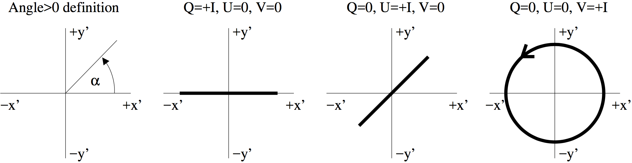
Fig. 6 The definition of the Stokes parameters used in RADMC-3D, which is consistent
with the IAU 1974 definitions (see Hamaker & Bregman (1996) A&AS 117,
pp.161). First panel shows that positive angle means counter-clockwise. In
the second to fourth panels the fat lines show how the tip of the real
electric field vector goes as a function of time for an observer at a fixed
location in space watching the radiation. The radiation moves toward the
reader. We call the second panel (\(Q=+I\)) ‘horizontally polarized’, the
third panel (\(U=+I\)) ‘diagonally polarized by +45 degrees’ and the
fourth panel (\(V=+I\)) ‘right-handed circularly polarized’. In the
images produced by RADMC-3D (image.out, see Section OUTPUT: image.out or image_****.out
and Fig. Fig. 9) the \(x'\) direction is the horizontal
direction and the \(y'\) direction is the vertical direction.
We can put these definitions into the standard formulae:
The angle \(\chi\) is the angle of the E-field in the \((x',y')\) coordinates, measured counter-clockwise from \(x'\) (consistent with our definition of angles). Example: \(\chi\) = 45 deg = \(\pi/4\), then \(\cos(2\chi)=0\) and \(\sin(2\chi)=1\), meaning that \(Q=0\) and \(U/I=+1\). Indeed this is consistent with the above definition that \(U/I=+1\) is \(E_x'=E_y'\).
The angle \(2\beta\) is the phase difference between the \(y'\)-component of the E-field and the \(x'\)-component of the E-field such that for \(0<\beta<\pi/2\) the E-field rotates in a counter-clockwise sense. In other words: the \(y'\)-wave lags \(2\beta\) behind the \(x'\) wave. Example: if we have \(\beta=\pi/4\), i.e. \(2\beta=\pi/2\), then \(\cos(2\beta)=0\) and \(\sin(2\beta)=1\), so we have \(Q=U=0\) and \(V/I=+1\). This corresponds to the \(y'\) wave being lagged \(\pi/2\) behind the \(x'\) wave, meaning that we have a counter-clockwise rotation. If we use the right-hand-rule and point the thumb into the direction of propagation (toward us) then the fingers indeed point in counter-rotating direction, meaning that \(V/I=+1\) is righthanded polarized radiation.
In terms of the real electric fields of a plane monochromatic wave:
(with \(E_h>0\) and \(E_v>0\) and \(\Delta_{h,v}\) are the phase lags of the components with respect to some arbitrary phase) we can write the Stokes components as:
with \(\Delta = \Delta_v - \Delta_h = 2\beta\).
In terms of the {em complex} electric fields of a plane monochromatic wave (the sign before the \(i\omega t\) is important):
(with \(E_h>0\) and \(E_v>0\) real numbers and \(\Delta_{h,v}\) are the phase lags of the components with respect to some arbitrary phase) we can write the Stokes components as:
Our conventions compared to other literature
The IAU 1974 definition is different from the definitions used in the Planck mission, for instance. So be careful. There is something said about this on the website of the healpix software http://healpix.jpl.nasa.gov/html/intronode12.htm .
Our definition is also different from the Mishchenko book and papers (see below). Compared to the books of Mishchenko and Bohren & Huffman, our definitions are:
As you see: only the \(U\) and \(V\) change sign. For a \(4\times 4\) Müller matrix \(M\) this means that the \(M_{II}\), \(M_{IQ}\), \(M_{QI}\), \(M_{QQ}\), as well as the \(M_{UU}\), \(M_{UV}\), \(M_{VU}\), \(M_{VV}\) stay the same, while \(M_{IU}\), \(M_{IV}\), \(M_{QU}\), \(M_{QV}\), as well as \(M_{UI}\), \(M_{UQ}\), \(M_{VI}\), \(M_{VQ}\) components would flip sign.
Compared to Mishchenko, Travis & Lacis book, what we call \(x'\) they call \(\theta\) and what we call \(y'\) they call \(\phi\). In their Figure 1.3 (which describes the definition of the Stokes parameters) they have the \(\theta\) direction pointing downward, rather than toward the right, i.e. rotated by 90 degrees clockwise compared to RADMC-3D. However, since RADMC-3D does not know what ‘right’ or ‘down’ are (only what \(x'\) and \(y'\) are) this rotation is merely a difference in how we plot things in a figure, and has no consequences for the results, as long as we define how \(x'\) and \(y'\) are oriented compared to our model (see Fig. Fig. 9 where \(x_{\mathrm{image}}\) is our \(x'\) here and likewise for \(y'\)).
Bohren & Huffman have the two unit vectors plotted in the following way: \({\bf e}_{\parallel}\) is plotted horizontally to the left and \({\bf e}_{\perp}\) is plotted vertically upward. Compared to us, our \(x'\) points toward {em minus} their \({\bf e}_{\parallel}\), while our \(y'\) points toward their \({\bf e}_{\perp}\), but since they plot their \({\bf e}_{\parallel}\) to the left, the orientation of our plot and their plots are consistent (i.e. if they say ‘pointing to the right’, they mean the same direction as we). But their definition of ‘right-handed circular polarization’ (clockwise when seen toward the source of the radiation) is our ‘left handed’.
The book by Wendisch & Yang ‘Theory of Atmospheric Radiative Transfer’ uses the same conventions as Bohren & Huffman, but their basis vector \({\bf e}_{\parallel}\) is plotted vertically and \({\bf e}_{\perp}\) is plotted horizontally to the right. This only affects what they call ‘horizontal’ and ‘vertical’ but the math stays the same.
Our definition is identical to the one on the English Wikipedia page on Stokes parameters http://en.wikipedia.org/wiki/Stokes_parameters (on 2 January 2013), with the only exception that what they call ‘righthanded’ circularly polarized, we call ‘lefthanded’. This is just a matter of nomenclature of what is right/left-handed, and since RADMC-3D does not know what ‘right/lefthanded’ is, this difference has no further consequences. Note, however, that the same Wikipedia page in different languages use different conventions! For instance, the German version of the page (on 2 January 2013) has the same Q and U definitions, but has the sign of V flipped.
Note that in RADMC-3D we have no global definition of the orientation of \(x'\) and \(y'\) (see e.g. Section Defining orientation for non-observed radiation). If we make an image with RADMC-3D, then the horizontal (x-) direction in the image corresponds to \(x'\) and the vertical (y-) direction corresponds to \(y'\), just as one would expect. So if you obtain an image from RADMC-3D and all the pixels in the image have \(Q=I\) and \(U=V=0\), then the electric field points horizontally in the image.
Defining orientation for non-observed radiation
To complete our description of the Stokes parameters we still need to define in which direction we let \(x'\) and \(y'\) point if we do not have an obvious observer, i.e. for radiation moving through our object of interest which may never reach us. In the Monte Carlo modules of RADMC-3D, when polarization is switched on, any photon package does not only have a wavelength \(\lambda\) and a direction of propagation \({\bf n}\) associated with it, but also a second unit vector \({\bf S}\), which is always assured to obey:
This leaves, for a given \({\bf n}\), one degree of freedom (any direction as long as it is perpendicular to \({\bf n}\)). It is irrelevant which direction is chosen for this, but whatever choice is made, it sets the definitions of the \(x'\) and \(y'\) directions. The definitions are:
So for \(Q=-I\), \(U=V=0\) the electric field points in the direction of \({\bf S}\), while for \(Q=+I\), \(U=V=0\) it is perpendicular to both \({\bf n}\) and \({\bf S}\).
However, if you are forced to change the direction of \({\bf S}\) for whatever reason, the Stokes components will also change. This coordinate transformation works as follows. We can transform from a ‘-basis to a ‘’-basis by rotating the \({\bf S}\)-vector counter-clockwise (as seen by the observer watching the radiation) by an angle \(\alpha\). Any vector \((x',y')\) in the ‘-basis will become a vector \((x'',y'')\) in a ‘’-basis, given by the transformation:
NOTE: We choose \((x',y')\) to be the usual counter-clockwise basis for the observer seeing the radiation. Rotating the basis in counter-clockwise direction means rotating the vector in that basis in clockwise direction, hence the sign convention in the matrix.
If we have \((I,Q,U,V)\) in the ‘-basis (which we might have written as \((I',Q',U',V')\) but by convention we drop the ‘), the \((I'',Q'',U'',V'')\) in the ‘’-basis becomes
Polarized scattering off dust particles: general formalism
Suppose we have one dust particle of mass \(m_{\mathrm{grain}}\) and we place it at location \({\bf x}\). Suppose this particle is exposed to a plane wave of electromagnetic radiation pointing in direction \({\bf n}_{\mathrm{in}}\) with a flux \({\bf F}_{\mathrm{in}}=F_{\mathrm{in}}\,{\bf n}_{\mathrm{in}}\). This radiation can be polarized, so that \(F_{\mathrm{in}}\) actually is a Stokes vector:
This particle will scatter some of this radiation into all directions. What will the flux of scattered radiation be, as observed at location \({\bf y}\neq{\bf x}\)? Let us define the vector
its length
and the unit vector
We will assume that \(r\gg a\) where \(a\) is the particle size. We define the {em scattering matrix elements} \(Z_{ij}\) (with \(i,j\) = \(1,2,3,4\)) such that the measured outgoing flux from the particle at \({\bf y}\) is
The values \(Z_{ij}\) depend on the direction into which the radiation is scattered (i.e. \({\bf e}_r\)) and on the direction of the incoming flux (i.e. \({\bf n}\)), but not on \(r\): the radial dependence of the outgoing flux is taken care of through the \(1/r^2\) factor in the above formula.
Some notes about our conventions are useful at this place. In many books the ‘scattering matrix’ is written as \(F_{ij}\) instead of \(Z_{ij}\), and is defined as the \(Z_{ij}\) for the case when radiation comes from one particular direction: \({\bf n}=(0,0,1)\). In this manual and in the RADMC-3D code, however, we will always write \(Z_{ij}\), because the symbol \(F\) can be confused with flux. The normalization of these matrix elements is also different in different books. In our case it has the dimension \(\mathrm{cm}^2\;\mathrm{gram}^{-1}\;\mathrm{ster}^{-1}\). The conversion from the conventions of other books is (where \(k=2\pi/\lambda\) is the wave number in units of 1/cm):
except that for the \(Z_{13}\), \(Z_{14}\), \(Z_{23}\), \(Z_{24}\), \(Z_{31}\), \(Z_{41}\), \(Z_{32}\), \(Z_{42}\) elements (if non-zero) there must be a minus sign before the \(Z_{ij,\mathrm{RADMC-3D}}\) because of the opposite \(U\) and \(V\) sign conventions (see Section Our conventions compared to other literature).
Note that the \(S_{ij,\mathrm{BohrenH}}\) are the matrix elements obtained
from the famous BHMIE.F code from the Bohren & Huffman book
(see Chapter Acquiring opacities from the WWW).
Polarized scattering off dust particles: randomly oriented particles
In the special case in which we either have spherical particles or we average over a large number of randomly oriented particles, the \(Z_{ij}\) elements are no longer dependent on both \({\bf e}_r\) and \({\bf n}\) but only on the angle between them:
So we go from \(Z_{ij}({\bf n},{\bf e}_r)\), i.e. a four-angle dependence, to \(Z_{ij}(\theta)\), i.e. a one-angle dependence.
Now let us also assume that there is no netto helicity of the particles (they are either axisymmetric or there exist equal amounts of particles as their mirror symmetric counterparts). In that case (see e.g. Mishchenko book) of the 16 matrix elements only 6 are non-zero and independent:
This is the case for scattering in RADMC-3D. Note that in Mie scattering the number of independent matrix elements reduces to just 4 because then \(Z_{22}=Z_{11}\) and \(Z_{44}=Z_{33}\). But RADMC-3D also allows for cases where \(Z_{22}\neq Z_{11}\) and \(Z_{44}\neq Z_{33}\), i.e. for opacities resulting from more detailed calculations such as DDA or T-matrix calculations.
Now, as described above, the Stokes vectors only have meaning if the directions of \(x'\) and \(y'\) are well-defined. For Eq. (eq-scatmat-for-randorient-nohelic) to be valid (and for the correct meaning of the \(Z_{ij}\) elements) the following definition is used: Before the scattering, the \({\bf S}\)-vector of the photon package is rotated (and the Stokes vectors accordingly transformed) such that the new \({\bf S}\)-vector is perpendicular to both \({\bf n}\) and \({\bf e}_r\). In other words, the scattering angle \(\theta\) is a rotation of the photon propagation around the (new) \({\bf S}\)-vector. The sign convention is such that
In other words, if we look into the incoming light (with \(z'\) pointing toward us), then for \(\sin(\theta)>0\) the photon is scattered into the \(x'>0\), \(y'=0\) direction (i.e. for us it is scattered to the right). The \({\bf S}\) vector for the outgoing photon remains unchanged, since the new \({\bf n}\) is also perpendicular to it.
So what does this all mean for the opacity? The scattering opacity tells us how much of the incident radiation is removed and converted into outgoing scattered radiation. The absorption opacity tells us how much of the incident radiation is removed and converted into heat. For randomly oriented particles without netto helicity both opacities are independent of the polarization state of the radiation. Moreover, the thermal emission is unpolarized in this case. This means that in the radiative transfer equation the extinction remains simple:
where \(I_I\), \(I_Q\), \(I_U\), \(I_V\) are the intensities (\(\mathrm{erg}\,\mathrm{s}^{-1}\,\mathrm{cm}^{-2}\,\mathrm{Hz}^{-1}\,\mathrm{ster}^{-1}\)) for the four Stokes parameters, and likewise for \(j_{\mathrm{emis}}\) and \(j_{\mathrm{scat}}\), and finally, \(s\) the path length along the ray under consideration. Note that if we would allow for fixed-orientation dust particles (which we don’t), Eq. (eq-radtrans-randomorient) would become considerably more complex, with extinction being matrix-valued and thermal emission being polarized.
Since \(\kappa_{\mathrm{scat}}\) converts incoming radiation into outgoing scattered radiation, it should be possible to calculate \(\kappa_{\mathrm{scat}}\) from angular integrals of the scattering matrix elements. For randomly oriented non-helical particles we indeed have:
where \(\mu=\cos\theta\). In a similar exercise we can calculate the anisotropy factor \(g\) from the scattering matrix elements:
This essentially completes the description of scattering as it is implemented in RADMC-3D.
We can precalculate the \(Z_{ij}(\theta)\) for every wavelength and for a
discrete set of values of \(\theta\), and store these in a table. This is
indeed the philosophy of RADMC-3D: You have to precompute them using, for
instance, the Mie code of Bohren and Huffman (see Chapter
Acquiring opacities from the WWW for RADMC-3D compliant wrappers around that
code), and then provide them to RADMC-3D through a file called
dustkapscatmat_xxx.inp (where xxx is the name of the dust species) which
is described in Section The dustkapscatmat_*.inp files. This file provides not
only the matrix elements, but also the \(\kappa_{\mathrm{abs}}\),
\(\kappa_{\mathrm{scat}}\) and \(g\) (the anisotropy factor). RADMC-3D
will then internally check that Eqs.(eq-scatmat-selfconsist-kappa,
eq-scatmat-selfconsist-g) are indeed fulfilled. If not, an error message
will result.
One more note: As mentioned in Section Definitions and conventions for Stokes vectors, the sign conventions of the Stokes vector components we use (the IAU 1974 definition) are different from the Bohren & Huffman and Mishchenko books. For randomly oriented particles, however, the sign conventions of the \(Z\)-matrix elements are not affected, because those matrix elements that would be affected are those that are in the upper-right and lower-left quadrants of the matrix, and these elements are anyway zero. So we can use, for randomly oriented particles, the matrix elements from those books and their computer codes without having to adjust the signs.
Scattering and axially symmetric models
In spherical coordinates it is possible in RADMC-3D to set up axially symmetric
models. The trick is simply to set the number of \(\phi\) coordinate points
nphi to 1 and to switch off the \(\phi\)-dimension in the grid (see
Section INPUT (required): amr_grid.inp). For isotropic scattering this mode has always
been implemented. But for anisotropic scattering things become more complex. For
such a model the scattering remains a fully 3-D problem: the scattering source
function has to be stored not only as a function of \(r\) and
\(\theta\), but also as a function of \(\phi\) (for a given observer
vantage point). The reason is that anisotropic scattering {em does} care about
viewing angle (in contrast to isotropic scattering). So even though for an
axisymmetric model the density and temperature functions only depend on
\(r\) and \(\theta\) (and are therefore mathematically 2-D), the
scattering source function depends on \(r\), \(\theta\) and
\(\phi\).
For this reason anisotropic scattering was, until version 0.40, not allowed for
2-D axisymmetric models. As of version 0.41 it is now possible to use the full
polarized scattering mode (scattering_mode=5) also for 2-D axisymmetric
models. The intermediate scattering modes (scattering_mode=2, 3, 4) remain
incompatible with 2-D axisymmetry. Isotropic scattering remains, as before,
fully compatible with 2-D axisymmetry.
One note of explanation: the way the full scattering is now implemented into
the case of 2-D axisymmetry is the following: internally we compute not just
the scattering source function for one angle, but for a whole set of \(\phi\)
angles (even though the grid has no \(\phi\)-points). Each time a photon in
the scattering Monte Carlo simulation enters a cell (which in 2-D
axisymmetry is an annulus), a loop over 360 \(\phi\) angles is performed, and
the scattering source function is computed for all of these angles. {em
This makes the code rather slow for each photon package!} But one needs
fewer photon packages to get sufficiently high signal-to-noise ratio. You
can experiment with fewer \(\phi\) angles by adding, in radmc3d.inp,
the following line (as an example):
dust_2daniso_nphi = 60
in which case instead of 360 the model will only use 60 \(\phi\) points. That will speed up the code significantly, but of course will treat the \(\phi\)-dependence of the scattering source function with lower precision.
For now the 2-D axisymmetric version of full scattering is only possible with first-order integration.
More about photon packages in the Monte Carlo simulations
In the ‘standard’ Monte Carlo approach, the input energy (e.g. starlight or, for the scattering Monte Carlo, the thermal emission of dust) is divided into \(N\) equal energy packages of photons, which then travel through the model and eventually either escape or get destroyed. This equal division scheme is, however, problematic for some model setups. For instance, if you have stars with vastly different luminosity in the model, then the brightest of these stars will dominate, by far, the number of output photon packages. This means that the material around low-brightness stars (which, by their proximity to these low-brightness stars, are still dominated by heating by these low-brightness stars) will experience very bad photon statistics.
To avoid this problem, RADMC-3D has, by default, its ‘weighted photon package mode’ switched on. This will make sure that each source of energy (i.e. each star, but also each other type of source) emits the same amount of photons. Only: bright stars will emit more energetic photon packages than dim stars.
The ‘weighted photon package mode’ will also solve another problem. Suppose a star lies far outside of the grid. It will emit most of its photons in directions that completely miss the grid. This means that RADMC-3D would waste a lot of time drawing random numbers for photons that will anyway not affect the model. Also here the ‘weighted photon package mode’ solves the problem: It will focus the photon packages toward the model grid, and lower their energy to compensate for their favorable focusing toward the grid.
NOTE: You can switch the mode off by setting mc_weighted_photons=0 in the
radmc3d.inp file.
Polarized emission and absorption by aligned grains
NOTE: This mode is still in the testing phase
Grain alignment and its effects on radiative transfer is a complex topic. A review is e.g. Andersson, B.G., Lazarian, A., & Vaillancourt, J.E. (2015) ‘Interstellar Dust Grain Alignment’, Annual Review of Astronomy and Astrophysics, 53(1), 501–539. In RADMC-3D grain alignment is included only in a limited form. First and foremost: RADMC-3D does not know about the physics {em causing} the grain alignment. You, the user, will have to tell how the grain are aligned by giving the code a directional vector field and for each wavelength the degree to which the grain is aligned to that directional vector (more on this later). This is according to the RADMC-3D philosophy of doing {em only} the radiative transfer and leaving the physics of the material to the user.
Basics
Suppose we have flattened (oblate) ellipsoidal grains with one axis of symmetry and no helicity. (While helicity may be needed to radiatively spin up grains, we assume that on average the helicity of the grains is zero.). Let us assume that they are aligned with that symmetry axis along the \(y\)-axis. We view radiation from the point where the \(z\)-axis points toward us. Horizontally polarized light (which has \(E\)-field in horizontal direction, i.e. in \(x\)-direction) has \(Q/I=+1\), vertically polarized light (with the \(\vec E\) vector aligned with the symmetry axis of the grain) has \(Q/I=-1\). We can then assume that the dust has different extinction coefficients for the horizontal and vertical axis. Let us call these:
We can define \(I\), \(Q\), \(U\) and \(V\) in terms of the electric field components \(E_x\) and \(E_y\). The electric field components for a perfectly coherent wave can be written as
where \(\Delta_x\) and \(\Delta_y\) are phase lags. The phase lag between the \(y\) and \(x\)-fields is \(\Delta=\Delta_y-\Delta_x\), meaning that for positive \(\Delta\) the \(y\)-field lags behind the \(x\)-field. We then define the Stokes components as:
Note that for \(V=I\) (\(\Delta=\pi/2\), i.e. the \(E_y\) lags \(\pi/2\) behind \(E_x\)) we have right-handed circularly polarized light, meaning that the tip of the \(\vec E\) field at a fixed point in space, when looking into the light (the propagation of light is toward the reader) rotates counter-clockwise (when the \(x\)-coordinate points right, and the \(y\)-coordinate points up). The 3-D helix of his field will be {em left-handed} (when the z-coordinate points into the propagation direction of the light, i.e. toward the reader, i.e. a right-handed coordinate system). For \(Q=I\) we have linearly polarized light in which the \(\vec E\)-field lies in the \(x\)-direction. For \(U=I\) we have linearly polarized light in which \(\vec E\) lies along the \(x=y\) line (when looking into the light). These definitions are consistent with the IAU 1974 definitions (Hamaker & Bregman 1996, A&AS 117, pp.161).
The \(E_x\) and \(E_y\) get absorbed in the following way:
where \(s\) is a length along the ray.
For this kind of problem it is convenient to introduce the so-called modified Stokes parameters \(I_{\mathrm{h}}\) and \(I_{\mathrm{v}}\):
so that we have
so that one can say, for perfectly coherent light,
With this we get the following extinction law:
How do \(U\) and \(V\) extinct? If we use Eqs. (eq-def-stokes-u, eq-def-stokes-v), and assume that the phase lag \(\Delta\) will not change during the extinction, then
This means that
and
In matrix notation
If we translate this to the usual Stokes components we get
with
The emission will be also independently in horizontal and vertical direction. But nothing will be emitted in U or V direction. So it is most convenient to express the emission/absorption process in terms of the modified Stokes parameters:
In terms of matrix notation this becomes
In terms of the normal Stokes parameters this becomes
or written slightly differently:
So to sum things up: We need only the absorption opacity for light with \(\vec E\) perpencidular to the symmetry axis (\(\kappa_{\mathrm{abs},\nu,h}\)) and the absorption opacity for light with \(\vec E\) parallel to the symmetry axis (\(\kappa_{\mathrm{abs},\nu,v}\)).
Implementation in RADMC-3D
Polarized emission in the images and spectra
When creating images (and spectra) the camera module of RADMC-3D
performs a ray-tracing calculation (‘volume rendering’) through the grid.
Normally (for randomly oriented grains) the extinction along the line of
sight is always unpolarized, i.e. each Stokes component is extincted
equally much. The thermal emission along the line of sight is also
unpolarized.
Now, however, we wish to include the effect of grain alignment in the ray-tracing. We assume that at position \(\vec x\) in the grid our oblate grain is aligned such that the minor axis points in the direction of the orientation vector \(\vec n_{\mathrm{align}}(\vec x)\). If the grain is prolate, we assume that it spins along one of its minor axes such that this spin axis is pointing along \(\vec n_{\mathrm{align}}(\vec x)\), so that, in effect, it acts as if it were an oblate grain again. In practice the alignment vector \(\vec n_{\mathrm{align}}(\vec x)\) does not lie always in the plane of the sky of the observer. Instead it will have an angle \(\theta\) with the line-of-sight direction vector \(\vec n_{\mathrm{los}}\) (note that this \(\theta\) angle is different from the scattering angle \(\theta\)), defined as
Here we assume that the grains have top/bottom symmetry so that we only have to concern ourselves with the positive values of \(\cos\theta\), hence the \(||\). If \(\cos\theta=1\) then we see the oblate grain from the top or the bottom, so that we do not expect any polarized emission. The strongest polarized emission is expected when \(\cos\theta=0\), which means that the oblate grain is seen edge-on.
We can now define the ‘projected alignment vector’ \(\vec n_{\mathrm{align,proj}}\), which is the alignment vector projected into the image plane:
To use the equations from Section Basics we must first rotate our image plane coordinates \((x,y)\) to new coordinates \((x',y')\) such that the \(y'\) (vertical) direction points along the \(\vec n_{\mathrm{align,proj}}\) vector while the \(x'\) (horizontal) direction points perpendicular to it. Let us write the Stokes vector of the radiation along the line of sight \((I_{\mathrm{in}},Q_{\mathrm{in}},U_{\mathrm{in}},V_{\mathrm{in}})\), where we implicitly know that these are also a function of frequency \(\nu\). This Stokes vector is defined with respect to the vector \(\vec S\) which is perpendicular to the line-of-sight direction vector \(\vec n_{\mathrm{los}}\) and defines the direction in which the \(y\)-coordinate of the image plane points. We must now express this incoming radiation (at the start of the segment) in the new \((x',y')\) image plane coordinates, i.e. with respect to the new vector \(\vec S'\) that points along \(\vec n_{\mathrm{align,proj}}\) (i.e. \(\vec S'\) is the normalized version of \(\vec n_{\mathrm{align,proj}}\)). This rotation is performed using
where \(\alpha\) is the angle between \(\vec S'\) and \(\vec S\) such that if (as seen by the observer) \(\vec S'\) lies counter-clockwise from \(\vec S\), \(\alpha\) is positive (the usual definition). With this new Stokes vector \((I',Q',U',V')\) we will now use the equations of Section Basics.
To be able to perform this rotation in a uniquely defined way, it is necessary that along each segment along the line of sight this new \((x',y')\) orientation stays fixed (but can vary from segment to segment). As the line-of-sight ray enters a cell and leaves it again, this line element (segment) will have its image-plane coordinates rotated according to the alignment vector of that cell. As a result, the integration must be done first order (assuming all source terms to be constant along the segment). In principle second order integration would also be possible, but then the trick with the rotation of the image coordinate plane such that \(y'\) points along the orientation vector does no longer work, and the integration of the formal transfer equation would become much more complex, involving the full Müller matrix formulation. We will not do this, so we will stick to first order integration of Eq. eq-formal-rt-emisabs-in-rotated-system.
For convenience we will leave out the primes (’) from here on, so while we write \((I,Q,U,V)\) we mean in fact \((I',Q',U',V')\). We now compute \(I_{\mathrm{h}}\) and \(I_{\mathrm{v}}\) using Eqs. (eq-modif-stokes-h, eq-modif-stokes-v). Now, along this segment of the ray, we can write Eq. eq-formal-rt-emisabs-in-rotated-system in the following form:
It becomes clear that it is easy to perform the first order integration of this equation along this ray segment:
where ‘start’ stands for the start of the ray segment, and ‘end’ the end of the ray segment (which becomes the start of the next ray segment), and \(\tau_h=\alpha_{\mathrm{h}}\Delta s\), \(\tau_v=\alpha_{\mathrm{v}}\Delta s\) and \(\tau_{uv}=\alpha_{\mathrm{uv}}\Delta s\), with \(\Delta s\) being the length of the segment.
We now compute \(I_{\mathrm{end}}\) and \(Q_{\mathrm{end}}\), and rotate back to the \((x,y)\) image plane coordinate system (i.e. using \(\vec S\) instead of \(\vec S'\) to define the Stokes parameters) by applying Eq. eq-rot-stokes-align but now with \(\alpha\rightarrow -\alpha\), and we have the values of the Stokes parameter at the end of the ray segment. Now we repeat this whole procedure for the next ray segment.
Polarized emission as source term in the Monte Carlo simulation
The polarization effects and anisotropic emission by aligned grains will also affect the Monte Carlo simulations.
For the thermal Monte Carlo (see Section The thermal Monte Carlo simulation: computing the dust temperature) this effect is not included. In principle it should be included, but it would slow the code down, and it is unlikely to play a significant role for the dust temperature, in particular since the anisotropy of thermal emission is not expected to be so strong (and the polarization state is irrelevant for computing the dust temperature). It is clear that we make a small error here, but we believe that this is well within the much stronger uncertainties of the dust opacities.
For the scattering Monte Carlo (see Section Scattered light in images and spectra: The ‘Scattering Monte Carlo’ computation), however, this effect may be important! The polarization caused by scattering of light off dust grains yields of course different results if the incident light is unpolarized or if it is already strongly polarized through, for instance, polarized thermal emission. In RADMC-3D this is therefore built into the scattering Monte Carlo. This will not slow down the code much because (in contrast to the thermal Monte Carlo) the polarized thermal emission only has to be computed at the start of each photon path, if the photon is emitted by the dust.
The way this is included is that when a photon is emitted by the dust inside a cell, RADMC-3D first randomly chooses which of the dust species emits the photon (the probabilities are weighted by the contribution each dust species makes to the emissivity at the given wavelength). Then the emission direction is randomly chosen, based on the \(\theta\)-dependent probability function (where \(\theta\) is the angle with the alignment direction) given by the average of the orthogonal (horizontal) and parallel (vertical) absorption opacities. Once the emission direction is chosen, the polarization state of the photon package is computed based on the orthogonal and parallel absorption opacities. Then the photon package is sent on its way.
Note that if alignment_mode = -1 then the polarized (and anisotropic)
thermal emission by aligned grains is only included in the ray-tracing for
images and spectra, while for alignment_mode = 1 it is also included
in the scattering Monte Carlo computation.
Consistency with other radiative processes
The above equations assume that the absorption/emission is the only radiative process included. However, in practice we also have other processes involved, such as line emission/absorption or the scattering source function. The way this can be treated here is to simply add these additional opacities to all four components of the extinction matrix of Eq. (eq-formal-rt-emisabs-in-rotated-system) and to add the additional emissivities to the vector with the Planck functions in Eq. (eq-formal-rt-emisabs-in-rotated-system). For the scattered light emissivity (which is a Stokes vector) we must also first perform a rotation from \(\vec S\) to \(\vec S'\) using the Stokes rotation formula of Eq. (eq-rot-stokes-align) before we add this emissivity to the equation. If we include the effect of alignment on the scattering (see Section Effect of aligned grains on the scattering) then also the scattering extinction will be different for the orthogonal (horizontal) and parallel (vertical) Stokes components. That is easy to include in this formalism.
Input files for RADMC-3D for aligned grains
In RADMC-3D we implement the functions \(\kappa_{\mathrm{abs},\nu,h}\) and \(\kappa_{\mathrm{abs},\nu,v}\) as a function of angle \(\theta\) which the alignment axis makes with the light of sight. For \(\theta\) we see the oblate grain from the top (face-on), so that there is no asymmetry between horizontal (orthogonal to the alignment orientation vector) and vertical (parallel to the alignment orientation vector). Then we will have \(\kappa_{\mathrm{abs},\nu,h}=\kappa_{\mathrm{abs},\nu,v}\). For \(\theta=90^{\circ}\) we will have the maximum difference between \(\kappa_{\mathrm{abs},\nu,h}\) and \(\kappa_{\mathrm{abs},\nu,v}\). We write
where \(k_{\nu,h}(\theta)\) and \(k_{\nu,v}(\theta)\) are dimensionless functions, and where we take \(\theta\in[0,90]\) (in degrees), or equivalently \(\cos(\theta)\in [0,1]\). We impose the condition that if we randomly orient this grain, the average opacity becomes the one we computed for the randomly oriented grains:
This yields the following integration condition on the dimensionless \(k_{\nu,h}\) and \(k_{\nu,v}\):
If we set, for all values of \(\theta\), \(k_{\nu,h}(\theta)=k_{\nu,v}(\theta)=1\) then we retrieve the result for spherical grains.
In RADMC-3D the functions \(k_{\nu,h}(\theta)\) and \(k_{\nu,v}(\theta)\)
are read in via the file dustkapalignfact_*.inp. This file
has the following structure:
# Any amount of arbitrary
# comment lines that tell which opacity this is.
# Each comment line must start with an # or ; or ! character
iformat                            <=== Typically 1 at present
nlam                               <=== Nr of wavelengths
nmu                                <=== Nr of angles sampled
lambda[1]                          <=== Wavelength grid in micron
...
lambda[nlam]
theta[1]                           <=== Angle grid in degrees
...
theta[nmu]
k_orth[1,1]       k_para[1,1]      <=== The arrays k_orth and k_para
...
k_orth[nmu,1]     k_para[nmu,1]
k_orth[1,2]       k_para[1,2]
...
k_orth[nmu,2]     k_para[nmu,2]
...
...
...
k_orth[1,nlam]    k_para[1,nlam]
...
k_orth[nmu,nlam]  k_para[nmu,nlam]
The angles theta are in degrees and must start at 0 and end at 90, or vice
versa. The nmu does not have to be the same (and the angles do not have to
be the same) as those in the dustkapscatmat_*.inp file. But the wavelength
grid must be identical to the one in the dustkapscatmat_*.inp file.
In order to make RADMC-3D read this file dustkapalignfact_*.inp the
dustopac.inp file should, for this particular dust species, have ‘20’ as the
way in which this dust species is read (instead of 10 which is used for
polarized scattering with the Z matrix).
In addition, RADMC-3D also needs to know the orientation direction of the grains. This is a vector field \(\vec p_{\mathrm{align}}(\vec x)\). The length of these vectors should be between 0 and 1, where 1 means that the grains are perfectly aligned and 0 means they are not aligned at all. The efficiency \(\epsilon_{\mathrm{align}}\) is thus given by
The directional unit-vector of alignment \(\vec n_{\mathrm{align}}(\vec x)\) is thus
The \(\vec p_{\mathrm{align}}(\vec x)\) vector field is in
the file grainalign_dir.inp (or its binary formatted version
grainalign_dir.binp). The format of this file is exactly the
same as that of the gas velocity file gas_velocity.inp. The
ascii format looks like:
iformat                                  <=== Typically 1 at present
nrcells
p_x[1]       p_y[1]       p_z[1]
..
p_x[nrcells] p_y[nrcells] p_z[nrcells]
Note that \(|\vec p_{\mathrm{align}}(\vec x)|\) should never be \(>1\). If it is found to be significantly \(>1\) at some point in the grid, then an error occurs. If it is only a tiny bit above 1, due to rounding errors, it will be normalized to 1.
The way in which partial alignment (\(0<\epsilon_{\mathrm{align}}<1\)) is treated in RADMC-3D is to treat the opacities and emissivities as simple linear sums of fully aligned and non aligned versions. For instance, Eqs. (eq-align-kappa-k-h, eq-align-kappa-k-v) then become
In order to tell RADMC-3D that it should include the effect of alignment on the
thermal emission of dust grains one must add a line in the radmc3d.inp file
with:
alignment_mode = 1
The example model in examples/run_simple_1_align/ demonstrates how the input
files have to be made to have RADMC-3D treat the aligned dust grains for thermal
emission.
Effect of aligned grains on the scattering
This is, currently, not yet implemented.
Grain size distributions
Quick summary of how to implement grain sizes
A common application of RADMC-3D is continuum radiative transfer in media with a grain size distribution. RADMC-3D does not know the concept of “grain size distribution”, and it does not care. You have to provide RADMC-3D will all the information it needs, such that it will handle the dust size distribution you want. All the responsibility lies with you, the user.
There are basically two ways by which you can make RADMC-3D treat a grain size distribution:
Method 1: Mixing the dust opacities into a single opacity file, having RADMC-3D think that there is only one dust species. Fast and simple.
Method 2: Computing \(N\) dust opacity files, having \(N\) independent dust species. Slower but more realistic and flexible.
In the following subsections we will discuss both methods.
Method 1: Size distribution in the opacity file (faster)
The simplest way is to compute a single dust opacity table (see Section
INPUT (required for dust transfer): dustopac.inp and dustkappa_*.inp or dustkapscatmat_*.inp or dust_optnk_*.inp) for a single dust species. You compute the weighted dust
opacity and put that into the file dustkappa_XXX.inp (for instance let’s
call it dustkappa_sizedistrib.inp) or dustkapscatmat_XXX.inp (for
instance let’s call it dustkapscatmat_sizedistrib.inp). All the information
about the size distribution shape is then encoded in this opacity file, and
RADMC-3D will never know that it is, in fact, a size distribution. The file
dust_density.inp will then only contain the spatial distribution of a single
grain species: that of the mixture of sizes. Advantage: it is the
easiest. Disadvantage: the size distribution will be identical
everywhere. Another disadvantage: each grain size will have the same temperature
(because RADMC-3D does not know that these are different dust sizes).
This method be useful to save computer time. You essentially do all the work of
computing the opacity of the size distribution beforehand (even before you start
RADMC-3D), so that you get a single opacity file that already contains the
size-distribution-weighted opacities. You must then be sure that you do the
weighting such that the opacity is “cross section per gram of dust”, where
“dust” is already the entire grain size distribution. The dust density in the
dust_density.inp file must then also be the density of the entire grain size
distribution. See Section The mathematics of grain size distributions for more
information about size distributions.
Method 2: Size distribution in the density file (better)
RADMC-3D can handle multiple dust species simultaneously and co-spatially. So
you can have \(N\) grain sizes, each represented by its own opacity file and
its own spatial density distribution. So if we, for example, have two sizes, 1
micron and 1 millimeter (i.e. \(N=2\)) then we would have, for instance, two
opacity files, dustkappa_1micron.inp and dustkappa_1mm.inp (don’t forget
to mark them both in dustopac.inp too), and within the dust_density.inp
file we have two density fields. This allows you, for instance, to have the
large grains near the midplane of a disk and the small grains vertically more
extended, because you can determine the density \(\rho\) of each dust
species completely independent from the others.
We have now two choices how to handle these species: (a) thermally coupled (set
itempdecoup = 0 in radmc3d.inp, see section INPUT: radmc3d.inp, or (b)
thermally decoupled (default, but you can set itempdecoup = 1 in
radmc3d.inp to make sure). The default is thermally decoupled, because that
is for most cases more realistic. If the grains are thermally decoupled, then,
in the optically thin regions exposed to hot stellar radiation, the small grains
tend to be hotter than the large ones. However, in optically thick regions the
small and large grains will tend to automatically acquire similar or the same
temperature(s).
Compared to the first method (with a single dust species), this method is more flexible (allowing different spatial distributions for different grain sizes) but also more costly (requiring the radiative transfer code to handle the interaction of the radiation with \(N\) independent dust species). You must then calculate each grain opacity file separately, and keep these normalized to “cross section per gram of this particular dust species or size”. Here, the weighting is not done in the opacity files, but in the fact that each grain size (or species) \(i\) has its own density \(\rho_i\). You would then need to make sure that these \(\rho_i\) are following the size distribution you wish. See Section The mathematics of grain size distributions for more information about size distributions.
The mathematics of grain size distributions
Grain size distributions can be confusing, so here is a small tutorial. Suppose we have the famous MRN (Mathis, Rumpl, Nordsieck) size distribution:
with \(a\) the radius of the grain, \(n(a)da\) the number of grains between sizes \(a\) and \(a+da\) per volume. We say that this powerlaw goes from \(a=a_{\mathrm{min}}\) to \(a=a_{\mathrm{max}}\), and we keep in mind that \(a_{\mathrm{max}}\) can be (but does not have to) orders of magnitude larger than \(a_{\mathrm{min}}\). The total dust density \(\rho\) is:
where \(m(a)\) is the mass of the grain:
where \(\rho_s\) is the material density of the grain material (typically somewhere between 1 and 3.6 \(\mathrm{gram}/\mathrm{cm}^3\), dependent on the material).
For RADMC-3D we have to disretize this into \(N\) bins. Since we can have \(a_{\mathrm{max}}\gg a_{\mathrm{min}}\), it is best to take a logarithmic grid in \(a\), i.e. equal spacing in \(\ln(a)\). So we divide the interval \([\ln(a_{\mathrm{min}}),\ln(a_{\mathrm{max}})]\) up into \(N\) equal size bins, numbering \(i=0\) to \(i=N-1\), with cell centers denoted as \(\ln(a_i)\) and the cell walls are denoted as \(\ln(a_{i-1/2})\) for the left- and \(\ln(a_{i+1/2})\) for the right-hand cell wall. We have \(\ln(a_{-1/2})=\ln(a_{\mathrm{min}})\) and \(\ln(a_{N-1/2})=\ln(a_{\mathrm{max}})\). For any \(i\) we have the same cell width in log-space: \(\Delta\ln(a)=\Delta\ln(a_i)=\ln(a_{i+1/2})-\ln(a_{i-1/2})\). Now the density for each bin is:
If the bin width \(\Delta\ln(a)\) is small enough, this can be approximated as
The total dust density is then
The opacity for bin \(i\) at some frequency \(\nu\) is approximately \(\kappa_\nu(a_i)\) if a small enough bin size is used. That means that the extinction coefficient
In method 2 (Section Method 2: Size distribution in the density file (better)) this is exactly what happens:
you specify \(N\) tables of \(\kappa_\nu(a_i)\) (each table containing all frequencies
for which you want to use the opacity), and the “mixing” happens in each grid cell on-the-fly
depending on the local values of \(\rho_i\). The values of \(\rho_i\) in the file
dust_density.inp are exactly these \(\rho_i\).
On the contrary, in method 1 (Section Method 1: Size distribution in the opacity file (faster)), you compute a nomalized \(\hat n(a_i)\) such that
so that with
we get
Now we can compute a grain-size-mean opacity:
which is computed before running RADMC-3D, and will be valid at all locations in the spatial grid. At each cell we only have the total dust density \(\rho\). The extinction coefficient is then