Main input and output files of RADMC-3D
RADMC-3D is written in fortran-90. It is written in such a way that the user
prepares input files (ending in .inp) for the program and then calls
radmc3d with some command-line options. The program then reads the input
files, and based on the command-line options will perform a certain calculation,
and finally outputs the results to output files (ending in .out) or
intermediate files (ending in .dat) which need further processing. In
principle the user therefore needs to compile the program only once, and can
then use the executable from that point onward. In this chapter we will describe
the various input/output and intermediate files and their formats. Just for
clarity: the Python routines in the python/ directory are only meant to make
it easier for the user to prepare the .inp files, and to make sense of the
.out and .dat files. They are not part of the main code radmc3d.
A few comments on RADMC-3D input and output files:
Most (though not all) files start with a format number. This number simply keeps track of the version of the way the information is stored the file. The idea is that if new versions of RADMC-3D come out in the future, it would be good to have the possibility that new information is added to the files. The format number is there to tell RADMC-3D whether a file is the new version or still an older version.
RADMC-3D has four types of I/O files:
Files ending with
.inpor.binpare input files that allow the user to specify to RADMC-3D which problem to solve.Files ending with
.dator.bdatare intermediate files that are typically created by RADMC-3D itself, but can also be read by RADMC-3D for further processing. For instance, the dust temperature is computed by the Monte Carlo method, but can also be read in later for ray-tracing.Files ending with
.outor.boutare final products of RADMC-3D, such as an image or spectrum.File ending with
.infoare small files containing some numbers that are useful to better interpret the output files of RADMC-3D. They are typically not very important for every-day use.
For many of the I/O files RADMC-3D can read and write formatted (i.e. text style: ascii) files, or binary files (i.e. C-style unformatted). This is specified by the file extension. See Chapter Binary I/O files for more details.
INPUT: radmc3d.inp
The radmc3d.inp file is a namelist file with the main settings for
RADMC-3D. The namelist is not a standard Fortran namelist style, but a simple
name = value list. If a name is not specified, the default values are taken.
So if the radmc3d.inp file is empty, then all settings are standard. Note
that some of these settings can be overwritten by command-line options! Here
is a non-exhaustive list of the variables that can be set.
incl_dust(default: depends on which input files are present)Normally RADMC-3D will recognize automatically whether dust continuum emission, absorption and scattering must be included: if e.g. a file called
dustopac.inpis present, it assumes that the dust must be included. But with this flag you can explicitly tell RADMC-3D whether it must be included (1) or not (0).incl_lines(default: depends on which input files are present)Normally RADMC-3D will recognize automatically whether line emission and absorption must be included: if e.g. a file called
lines.inpis present, it assumes that molecular/atomic lines must be included. But with this flag you can explicitly tell RADMC-3D whether it must be included (1) or not (0).nphotornphot_therm(default: 100000)The number of photon packages used for the thermal Monte Carlo simulation.
nphot_scat(default: 100000)The number of photon packages for the scattering Monte Carlo simulations, done before image-rendering.
nphot_spec(default: 10000)The number of photon packages for the scattering Monte Carlo simulations, done during spectrum-calculation. This is actually the same functionality as for
nphot_scat, but it is used (and only used) for the spectrum and SED calculations. The reason to have a separate value for this is that for spectra you may not need as many photon packages as for imaging, because you anyway integrate over the images. Many of the annoying ‘stripe noise’ in images when using insufficiently largenphot_scatwill cancel each other out in the flux calculation. Sonphot_specis usually taken smaller thannphot_scat.nphot_mono(default: 100000)The number of photon packages for the Monte Carlo simulations for the
mcmonocalculation (see Section Special-purpose feature: Computing the local radiation field).iseed(default: -17933201) [Fine-tuning only]A starting value of the random seed for the Monte Carlo simulation.
ifast(default: 0) [Fine-tuning only]By setting this to 1 or 2 you will get a faster Monte Carlo simulation, at the cost of being less accurate.
enthres(default: 0.01) [Fine-tuning only]This is the fraction by which the energy in each cell may increase before the temperature is recalculated in the Monte Carlo simulation. The smaller this value, the more accurate the thermal Monte Carlo simulation, but the more computationally costly. 0.01 has proven to be fine.
itempdecoup(default: 1)If set to 0, then the temperatures of all coexisting dust species are always forced to be the same. If 1, then each dust species is thermally independent of the other.
istar_sphere(default: 0)If 0 (=default), then all stars are treated as point-sources. If 1, then all stars are treated as finite-size spheres. This mode is more accurate and more realistic, but the applications are a bit more restricted. Such finite-size stars are (for technical reasons) not always allowed anywhere in the model. But for problems of circumstellar disks and envelopes in spherical coordinates, it is recommended to set this to 1. Typically, if a star is outside the grid (in spherical coordinates this can also be at the origin of the coordinate system, as long as the inner radius of the coordinate system is larger than the stellar radius!) the use of the finite-size star mode is always possible. But if the star is on the grid, there are technical limitations.
ntemp(default: 1000) [Fine-tuning only]The temperatures are determined in the Monte Carlo method using tabulated pre-computed integrals. This saves time. This is the number of temperatures for which this is precalculated. The temperatures are sampled in a logarithmic way, i.e. log(temp) is linearly equally spaced between log(temp0) and log(temp1), see below.
temp0(default: 0.01) [Fine-tuning only]The lowest pre-calculated temperature.
temp1(default: 1e5) [Fine-tuning only]The highest pre-calculated temperature.
scattering_mode_maxWhen
radmc3dreads the dust opacity files it checks if one or more of the opacity files has scattering opacity included. If yes, thescattering_modewill automatically be set to 1. It will also check if one or more includes anisotropic scattering. If yes, thescattering_modewill automatically be set to 2. But the user may nevertheless want to exclude anisotropic scattering or exclude scattering altogether (for instance for testing purposes, or if the user knows from experience that the scattering or anisotropic nature of scattering is not important for the problem at hand). Rather than editing the opacity files to remove the scattering and/or Henyey-Greenstein \(g\)-factors, you can limit the value thatradmc3dis allowed to makescattering_modeby setting the variablescattering_mode_max. If you setscattering_mode_max=0then no matter what opacity files you have, scattering will not be treated. If you setscattering_mode_max=1, then no matter what opacity files you have, scattering will be treated in an isotropic way.unformatted(Obsolete)rto_style(default=1)This determines whether the output of space-dependent data will be in ASCII form (
rto_style=1), f77-unformatted form (rto_style=2, obsolete) or binary form (rto_style=3). See Chapter Binary I/O files for details.camera_tracemode(default: 1)If
camera_tracemode=-1, the images that are rendered by RADMC-3D will instead by the column depth traced along each ray. Ifcamera_tracemode=-2, the images that are rendered by RADMC-3D will instead by the continuum optical depth traced along each ray. By defaultcamera_tracemode=1, which is the normal mode, where real images are being created.camera_nrrefine(default: 100)For images: to assure that flux is correctly sampled, the image pixels will not just be rendered one ray per pixel. Instead, if necessary, a pixel will spawn 2x2 sub-pixels recursively (each of which can split again into 2x2 until the required resolution is obtained) so as to assure that the flux in each pixel is correct.
camera_nrrefinetells how deep RADMC-3D is allowed to recursively refine. 100 is therefore effectively infinite. Putting this to 0 means that you go back to 1 ray per pixel, which is fast, but may seriously misrepresent the flux in each pixel. See Section The issue of flux conservation: recursive sub-pixeling for more details.camera_refine_criterion(default: 1.0) [Fine-tuning only]Setting this value to smaller than 1 means that you refine the recursive pixeling until a tighter criterion is met. The smaller this value, the more accurate the fluxes in each pixel, but the longer it takes to render. See Section The issue of flux conservation: recursive sub-pixeling for more details.
camera_incl_stars(default: 1)If 0, then only the interstellar/circumstellar material is rendered for the images and spectra. If 1, then also the stellar flux is included in the spectra and images.
camera_starsphere_nrpix(default: 20) [Fine-tuning only]For rectangular images and for the spectra/SEDs (but not for spectra/SEDs created with circular pixel arrangements, see Section Circular images), this number tells RADMC-3D how much it should do sub-pixeling over the stellar surface. That is: 20 means that at least 20 sub-pixels are assured over the stellar surface. This is important for flux conservation (see Section The issue of flux conservation: recursive sub-pixeling).
camera_spher_cavity_relres(default: 0.05) [Fine-tuning only]Determines the size of sub-pixels inside the inner grid radius of spherical coordinates.
camera_localobs_projection(default: 1)(Only for local observer mode) The type of projection on the sphere of observation.
camera_min_dangle(default 0.05) [Fine-tuning only]Fine-tuning parameter for recursive subpixeling (see Section The solution: recursive sub-pixeling), for spherical coordinates, assuring that not too fine subpixeling would slow down the rendering of images or spectra too much.
camera_max_dangle(default 0.3) [Fine-tuning only]Fine-tuning parameter for recursive subpixeling (see Section The solution: recursive sub-pixeling), for spherical coordinates, preventing that too coarse subpixeling would reduce the accuracy.
camera_min_drr(default 0.003) [Fine-tuning only]Fine-tuning parameter for recursive subpixeling, for spherical coordinates, assuring that not too fine subpixeling would slow down the rendering of images or spectra too much.
camera_diagnostics_subpix(default: 0)Setting this to 1 forces RADMC-3D to write out a file called
subpixeling_diagnostics.outwhich contains four columns, for respectivly:px,py,pdx,pdy, i.e. the pixel position and its size. This is for all pixels, including the sub-pixels created during the recursive subpixeling procedure (Section The solution: recursive sub-pixeling). This allows the user to find out if the recursive subpixeling went well or if certain areas were over/under-resolved. This is really only meant as a diagnostic.camera_secondorder(default: 0)If set to 1, RADMC-3D will interpolate all emission/absorption quantities to the cell corners, and then use a second order integration routine with bilinear interpolation of the source terms to integrate the ray-tracing formal transfer equations. See Section Second order ray-tracing (Important information!) for more information about the second order integration: It is recommended to read it!
camera_interpol_jnu(default: 0) [Fine-tuning only]Fine-tuning parameter for ray-tracing, only used for when second order integration is done (i.e. if
camera_secondorder=1). If 0 (default), then the source function \(S_\nu\) is the one that is interpolated on the grid, while if 1, then the emissivity \(j_\nu\) is the one that is interpolated on the grid. The differences are minimal, but if strange results appear (when using second order integration) then you may want to experiment a bit with this parameter.mc_weighted_photons(default: 1) [Fine-tuning only]If
mc_weighted_photons=1 (default) then in Monte Carlo simulations not all photon packages will have the same energy (see Section More about photon packages in the Monte Carlo simulations). The energy will be weighted such that each star or emission mechanism will emit, on average, the same number of photon packages. As an example: If you have a stellar binary consisting of an O-star surrounded by a Brown Dwarf, but the Brown Dwarf is surrounded by a disk, then although the O star is much brighter than the O-star, the very inner regions of the Brown Dwarf disk is still predominantly heated by the Brown Dwarf stellar surface, because it is much closer to that material. If you do not have weighted photon packages, then statistically the Brown Dwarf would emit perhaps 1 or 2 photon packages, which makes the statistics of the energy balance in the inner disk very bad. Bymc_weighted_photons=1 both the Brown Dwarf and the O-star will each emit the same number of photon packages; just the energy of the photon packages emitted by the Brown Dwarf are much less energetic than those from the O-star. This now assures a good photon statistics everywhere.optimized_motion(default: 0) [Fine-tuning only]If
optimized_motionis set to 1, then RADMC-3D will try to calculate the photon motion inside cells more efficiently. This may save computational time, but since it is still not very well tested, please use this mode with great care! It is always safer not to use this mode.lines_mode(default: 1)This mode determines how the level populations for line transfer are computed. The default is 1, which means: Local Thermodynamic Equilibrium (LTE). For other modes, please consult Chapter Line radiative transfer.
lines_maxdoppler(default: 0.3) [Fine-tuning only]If the doppler catching mode is used (see Section Preventing doppler jumps: The ‘doppler catching method’), this parameter tells how fine RADMC-3D must sample along the ray, in units of the doppler width, when a line is doppler-shifting along the wavelength-of-sight.
lines_partition_ntempint(default 1000) [Fine-tuning only]Number of temperature sampling points for the internally calculated partition function for molecular/atomic lines.
lines_partition_temp0(default 0.1) [Fine-tuning only]Smallest temperature sampling point for the internally calculated partition function for molecular/atomic lines.
lines_partition_temp1(default 1E5) [Fine-tuning only]Largest temperature sampling point for the internally calculated partition function for molecular/atomic lines.
lines_show_pictograms(default 0)If 1, then print a pictogram of the levels of the molecules/atoms.
tgas_eq_tdust(default: 0)By setting
tgas_eq_tdust=1you tellradmc3dto simply read thedust_temperature.inpfile and then equate the gas temperature to the dust temperature. If multiple dust species are present, only the first species will be used.subbox_nx,subbox_ny,subbox_nz,subbox_x0,subbox_x1,subbox_y0,subbox_y1,subbox_z0,subbox_z1Parameters specifying the subbox size for the subbox extraction. See Section Making a regularly-spaced datacube (‘subbox’) of AMR-based models for details.
INPUT (required): amr_grid.inp
This is the file that specifies what the spatial grid of the model looks
like. See Chapter More information about the gridding. This file is essential, because most
other .inp and .dat files are simple lists of numbers which do not
contain any information about the grid. All information about the grid is
contained in the amr_grid.inp, also for non-AMR regular grids. Note that
in the future we will also allow for unstructured grids. The corresponding grid
files will then be named differently.
There are three possible AMR grid styles:
Regular grid: No mesh refinement. This is grid style 0.
Oct-tree-style AMR (‘Adaptive Mesh Refinement’, although for now it is not really ‘adaptive’). This is grid style 1.
Layer-style AMR. This is grid style 10.
Regular grid
For a regular grid, without grid refinement, the amr_grid.inp looks like:
iformat                                  <=== Typically 1 at present
0                                        <=== Grid style (regular = 0)
coordsystem
gridinfo
incl_x       incl_y       incl_z
nx           ny           nz
xi[1]        xi[2]        xi[3]       ........  xi[nx+1]
yi[1]        yi[2]        yi[3]       ........  yi[ny+1]
zi[1]        zi[2]        zi[3]       ........  zi[nz+1]
The meaning of the entries are:
iformat: The format number, at present 1. For unformatted files this must be 4-byte integer.coordsystem: Ifcoordsystem < 100the coordinate system is cartesian. If100 <= coordsystem < 200the coordinate system is spherical (polar). Cylindrical coordinates have not yet been built in in this version. For unformatted files this must be 4-byte integer.gridinfo: Ifgridinfo==1there will be abundant grid information written into this file, possibly useful for post-processing routines. Typically this is redundant information, so it is advised to setgridinfo=0to save disk space. In the following we will assume thatgridinfo=0. For unformatted files this must be 4-byte integer.incl_x,incl_y,incl_z: These are either 0 or 1. If 0 then this dimension is not active (so upon grid refinement no refinement in this dimension is done). If 1 this dimension is fully active, even if the number of base grid cells in this direction is just 1. Upon refinement the cell will also be splitted in this dimension. For unformatted files these numbers must be 4-byte integer.nx,ny,nz: These are the number of grid cells on the base grid in each of these dimensions. For unformatted files these numbers must be 4-byte integer.xi[1]...xi[nx+1]: The edges of the cells of the base grid in x-direction. Fornxgrid cells we havenx+1cell walls, hencenx+1cell wall positions. For unformatted files these numbers must be 8-byte reals (=double precision).yi[1]...yi[ny+1]: Same as above, but now for y-direction.zi[1]...zi[nz+1]: Same as above, but now for z-direction.
Example of a simple 2x2x2 regular grid in cartesian coordinates:
1
0
1
0
1  1  1
2  2  2
-1.  0. 1.
-1.  0. 1.
-1.  0. 1.
Oct-tree-style AMR grid
For a grid with oct-tree style grid refinement (see Section
Oct-tree Adaptive Mesh Refinement), the amr_grid.inp looks like:
iformat                                  <=== Typically 1 at present
1                                        <=== Grid style (1 = Oct-tree)
coordsystem
gridinfo
incl_x       incl_y       incl_z
nx           ny           nz
levelmax     nleafsmax    nbranchmax     <=== This line only if grid style == 1
xi[1]        xi[2]        xi[3]       ........  xi[nx+1]
yi[1]        yi[2]        yi[3]       ........  yi[ny+1]
zi[1]        zi[2]        zi[3]       ........  zi[nz+1]
(0/1)                   <=== 0=leaf, 1=branch (only if amrstyle==1)
(0/1)                   <=== 0=leaf, 1=branch (only if amrstyle==1)
(0/1)                   <=== 0=leaf, 1=branch (only if amrstyle==1)
(0/1)                   <=== 0=leaf, 1=branch (only if amrstyle==1)
(0/1)                   <=== 0=leaf, 1=branch (only if amrstyle==1)
(0/1)                   <=== 0=leaf, 1=branch (only if amrstyle==1)
(0/1)                   <=== 0=leaf, 1=branch (only if amrstyle==1)
(0/1)                   <=== 0=leaf, 1=branch (only if amrstyle==1)
(0/1)                   <=== 0=leaf, 1=branch (only if amrstyle==1)
...
...
The keywords have the same meaning as before, but in addition we have:
(0/1): NOTE: Only foramrstyle==1. These are numbers that are either 0 or 1. If 0, this means the current cell is a leaf (= a cell that is not refined and is therefore a ‘true’ cell). If 1, the current cell is a branch with 2 (in 1-D), 4 (in 2-D) or 8 (in 3-D) daughter cells. In that case the next (0/1) numbers are for these daughter cells. In other words, we immediately recursively follow the tree. The order in which this happens is logical. In 3-D the first daughter cell is (1,1,1), then (2,1,1), then (1,2,1), then (2,2,1), then (1,1,2), then (2,1,2), then (1,2,2) and finally (2,2,2), where the first entry represents the x-direction, the second the y-direction and the third the z-direction. If one or more of the daughter cells is also refined (i.e. has a value 1), then first this sub-tree is followed before continuing with the rest of the daughter cells. If we finally return to the base grid at some point, the next (0/1) number is for the next base grid cell (again possibly going into this tree if the value is 1). The order in which the base grid is scanned in this way is from1tonxin the innermost loop, from1tonyin the middle loop and from1tonzin the outermost loop. For unformatted files these numbers must be 4-byte integers, one record per number.
Example of a simple 1x1x1 grid which is refined into 2x2x2 and for which the (1,2,1) cell is refined again in 2x2x2:
1
1
1
0
1  1  1
1  1  1
10 100 100
-1.  1.
-1.  1.
-1.  1.
1
0
0
1
0
0
0
0
0
0
0
0
0
0
0
0
0
Layer-style AMR grid
For a grid with layer-style grid refinement (see Section
Layered Adaptive Mesh Refinement), the amr_grid.inp looks like:
iformat                                  <=== Typically 1 at present
10                                       <=== Grid style (10 = layer-style)
coordsystem
gridinfo
incl_x       incl_y       incl_z
nx           ny           nz
nrlevels     nrlayers                    <=== This line only if grid style == 10
xi[1]        xi[2]        xi[3]       ........  xi[nx+1]
yi[1]        yi[2]        yi[3]       ........  yi[ny+1]
zi[1]        zi[2]        zi[3]       ........  zi[nz+1]
parentid     ix  iy  iz   nx  ny  nz
parentid     ix  iy  iz   nx  ny  nz
parentid     ix  iy  iz   nx  ny  nz
parentid     ix  iy  iz   nx  ny  nz
.
.
.
The keywords have the same meaning as before, but in addition we have:
nrlevels: How many levels you plan to go, wherenrlevels==0means no refinement,nrlevels==1means one level of refinement (factor of 2 in resolution), etc.nrlayers: How many layers do you have, withnrlayers==0means no refinement,nrlayers==1means one layer of refinement (factor of 2 in resolution), etc.parentid: (For each layer) The parent layer for this layer.parentid==0means parent is base grid. First layer hasid==1.ix,iy,iz: (For each layer) The location in the parent layer where the current layer starts.nx,ny,nz: (For each layer) The size of the layer as measured in units of the the parent layer. So the actual size of the current layer will be (in 3-D):2*nx,2*ny,2*nz. In 2-D, with only the x- and y- dimensions active, we have a size of2*nx,2*nywith of course size 1 in z-direction.
As you can see, this is a much easier and more compact way to specify mesh refinement. But it is also less ‘adaptive’, as it is always organized in square/cubic patches. But it is much easier to handle for the user than full oct-tree refinement.
Note that this layer-style refinement is in fact, internally, translated into the oct-tree refinement. But you, as the user, will not notice any of that. The code will input and output entirely in layer style.
NOTE: The layers must be specify in increasing refinement level! So the first layer (layer 1) must have the base grid (layer 0) as its parent. The second layer can have either the base grid (layer 0) or the first layer (layer 1) as parent, etc. In other words: the parent layer must always already have been specified before.
Example of a simple 2-D 4x4 grid which has a refinement patch in the middle of again 4x4 cells (=2x2 on the parent grid), and a patch of 2x2 (=1x1 on the parent grid) starting in the upper left corner:
1
100
1
0
1  1  0
4  4  1
1  2
-2. -1. 0. 1. 2.
-2. -1. 0. 1. 2.
-0.5 0.5
0  2  2  1  2  2  1
0  1  1  1  1  1  1
This has just one level of refinement, but two patches at level 1.
Anothe example: two recursive layers. Again start with a 2-D 4x4 grid, now refine it in the middle with again a 4x4 sub-grid (=2x2 on the parent grid = layer 0) and then again a deeper layer of 4x4 (=2x2 on the parent grid = layer 1) this time starting in the corner:
1
100
1
0
1  1  0
4  4  1
2  2
-2. -1. 0. 1. 2.
-2. -1. 0. 1. 2.
-0.5 0.5
0  2  2  1  2  2  1
1  1  1  1  2  2  1
Note that with this layer-style grid, the input data will have to be speficied
layer-by-layer: first the base grid, then the first layer, then the second
etc. This is worked out in detail for dust_density.inp in Section
INPUT (required for dust transfer): dust_density.inp. This will include redundant data, because you specify the
data on the entire base grid, also the cells that later will be replaced by a
layer. Same is true for any layer that has sub-layers. The data that is
specified in these regions will be simply ignored. But for simplicity we do
still require it to be present, so that irrespective of the deeper layers, the
data in any layer (including the base grid, which is layer number 0) is simply
organized as a simple data cube. This redundancy makes the input and output
files larger than strictly necessary, but it is much easier to handle as each
layer is a datacube. For memory/hardisk-friendly storage you must use the
oct-tree refinement instead. The layers are meant to make the AMR much more
accessible, but are somewhat more memory consuming.
INPUT (required for dust transfer): dust_density.inp
This is the file that contains the dust densities. It is merely a list of
numbers. Their association to grid cells is via the file amr_grid.inp (see
Chapter Binary I/O files for the binary version of this file, which is more
compact). Each dust species will have its own density distribution, completely
independently of the others. That means that at each position in space several
dust species can exist, and the density of these can be fully freely
specified. The structure of this file is as follows. For formatted style
(dust_density.inp):
iformat                                  <=== Typically 1 at present
nrcells
nrspec
density[1,ispec=1]
..
density[nrcells,ispec=1]
density[1,ispec=2]
..
..
..
density[nrcells,ispec=nrspec]
Here nrspec is the number of independent dust species densities
that will be given here. It can be 1 or larger. If it is 1, then of course
the density[1,ispec=2] and following lines are not present
in the file. The nrcells is the number of cells. For different
kinds of grids this can have different meaning. Moreover, for different
kinds of grids the order in which the density values are given is also
different. So let us now immediately make the following distinction (See
Chapter More information about the gridding on the different kinds of grids):
For regular grid and oct-tree AMR grids:
The value of
nrcellsdenotes the number of true cells, excluding the cells that are in fact the parents of 2x2x2 subcells; i.e. the sum of the volumes of all true cells (=leafs) adds up to the volume of the total grid). The order of these numbers is always the same ‘immediate recursive subtree entry’ as in theamr_grid.inp(Section INPUT (required): amr_grid.inp).For layer-style AMR grids:
The value of
nrcellsdenotes the number of values that are specified. This is generally a bit more than the true number of cells specified in the oct-tree style AMR (see above). In the layer-style AMR mode you specify the dust density (or any other value) first at all cells of the base grid (whether a cell is refined or not does not matter), the at all cells of the first layer, then the second layer etc. Each layer is a regular (sub-)grid, so the order of the values is simply the standard order (same as for regular grids). This means, however, that the values of the density in the regular grid cells that are replaced by a layer are therefore redundant. See Section On the ‘successively regular’ kind of data storage, and its slight redundancy for a discussion of this redundancy. The main advantage of this layer-style grid refinement is that the input and output always takes place on regular grids and subgrids (=layers). This is much easier to handle than the complexities of the oct-tree AMR.
Example: dust_density.inp for a regular grid
Now let us look at an example of a dust_density.inp file,
starting with one for the simplified case of a regular 3-D grid (see
Sections Regular grid and Regular grids):
iformat                                  <=== Typically 1 at present
nrcells
nrspec
density[1,1,1,ispec=1]
density[2,1,1,ispec=1]
..
density[nx,1,1,ispec=1]
density[1,2,1,ispec=1]
..
..
density[nz,ny,nz,ispec=1]
density[1,1,1,ispec=2]
..
..
..
density[nz,ny,nz,ispec=nrspec]
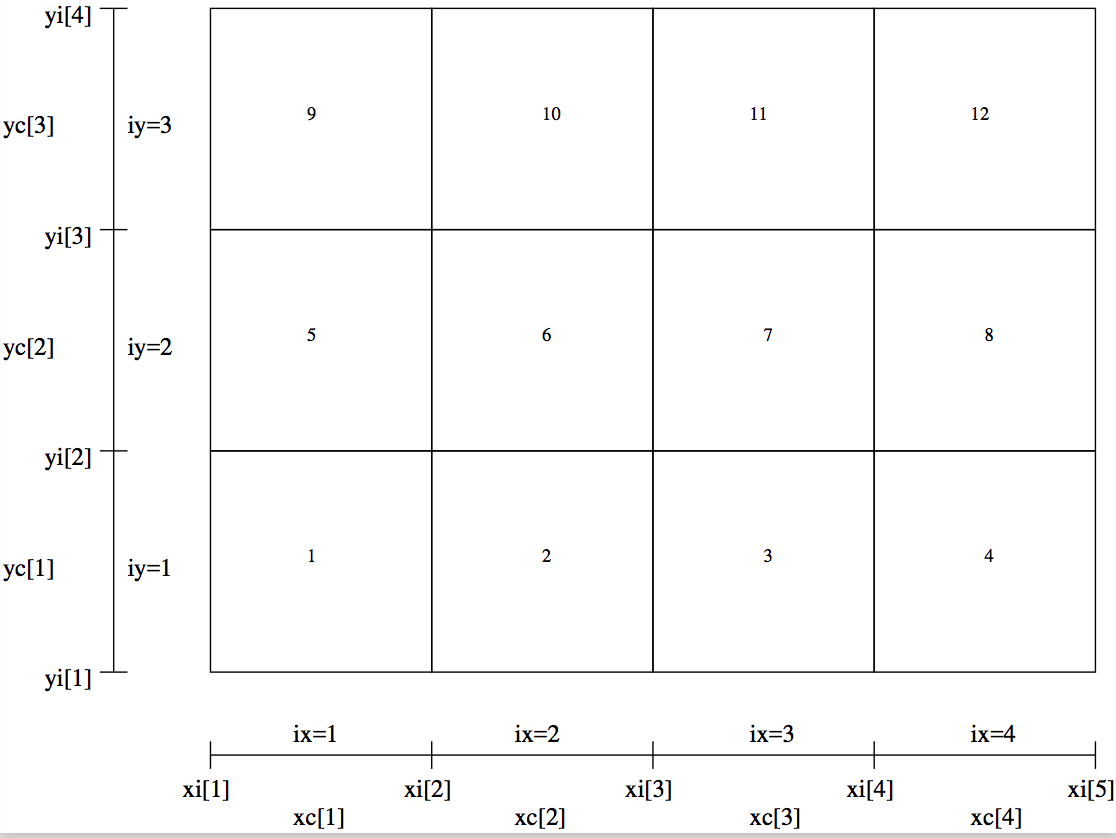
Fig. 31 Example of a regular 2-D grid with nx=4 and ny=3 (as
Fig. Fig. 21), with the order of the cells shown as
numbers in the cells.
Example: dust_density.inp for an oct-tree refined grid
For the case when you have an oct-tree refined grid (see Sections
Oct-tree-style AMR grid and Oct-tree Adaptive Mesh Refinement), the order of the
numbers is the same as the order of the cells as specified in the
amr_grid.(u)inp file (Section INPUT (required): amr_grid.inp). Let us take the
example of a simple 1x1x1 grid which is refined into 2x2x2 and for which the
(1,2,1) cell is refined again in 2x2x2 (this is exactly the same example as
shown in Section Oct-tree-style AMR grid, and for which the
amr_grid.inp is given in that section). Let us also assume that we have only
one dust species. Then the dust_density.inp file would be:
iformat                                  <=== Typically 1 at present
15                                       <=== 2x2x2 - 1 + 2x2x2 = 15
1                                        <=== Let us take just one dust spec
density[1,1,1]                           <=== This is the first base grid cell
density[2,1,1]
density[1,2,1;1,1,1]                     <=== This is the first refined cell
density[1,2,1;2,1,1]
density[1,2,1;1,2,1]
density[1,2,1;1,2,1]
density[1,2,1;1,1,2]
density[1,2,1;2,1,2]
density[1,2,1;1,2,2]
density[1,2,1;1,2,2]                     <=== This is the last refined cell
density[2,2,1]
density[1,1,2]
density[2,1,2]
density[1,2,2]
density[2,2,2]                           <=== This is the last base grid cell
A more complex example is shown in Fig. Example of a 2-D grid with oct-tree refinement (as Fig. fig-oct-tree-amr) with the order of the cells shown as numbers in the cells.. An unformatted version is also available, in the standard way (see above).
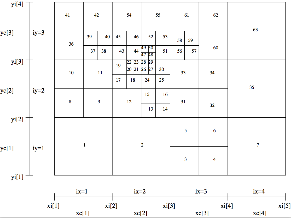
Fig. 32 Example of a 2-D grid with oct-tree refinement (as Fig. Example of a 2-D grid with oct-tree refinement. The base grid has nx=4 and ny=3. Three levels of refinement are added to this base grid.) with the order of the cells shown as numbers in the cells.
Example: dust_density.inp for a layer-style refined grid
For the case when you have an layer-style refined grid (see Sections
Layer-style AMR grid and Layered Adaptive Mesh Refinement) you specify the
density in a series of regular boxes (=layers). The first box is the base
grid, the second the first layer, the third the second layer etc. The value
nrcells now tells the combined sizes of the all the boxes. If we
take the second example of Section Layer-style AMR grid: a simple 2-D
4x4 grid which has a refinement patch (=layer) in the middle of again 4x4
cells, and again one patch of 4x4 this time, however, starting in the upper
left corner (see the amr_grid.inp file given in Section
Layer-style AMR grid), then the dust_density.inp file
has the following form:
iformat                                  <=== Typically 1 at present
48                                       <=== 4x4 + 4x4 + 4x4 = 48
1                                        <=== Let us take just one dust spec
density[1,1,1,layer=0]
density[2,1,1,layer=0]
density[3,1,1,layer=0]
density[4,1,1,layer=0]
density[1,2,1,layer=0]
density[2,2,1,layer=0]                   <=== This a redundant value
density[3,2,1,layer=0]                   <=== This a redundant value
density[4,2,1,layer=0]
density[1,3,1,layer=0]
density[2,3,1,layer=0]                   <=== This a redundant value
density[3,3,1,layer=0]                   <=== This a redundant value
density[4,3,1,layer=0]
density[1,4,1,layer=0]
density[2,4,1,layer=0]
density[3,4,1,layer=0]
density[4,4,1,layer=0]
density[1,1,1,layer=1]                   <=== This a redundant value
density[2,1,1,layer=1]                   <=== This a redundant value
density[3,1,1,layer=1]
density[4,1,1,layer=1]
density[1,2,1,layer=1]                   <=== This a redundant value
density[2,2,1,layer=1]                   <=== This a redundant value
density[3,2,1,layer=1]
density[4,2,1,layer=1]
density[1,3,1,layer=1]
density[2,3,1,layer=1]
density[3,3,1,layer=1]
density[4,3,1,layer=1]
density[1,4,1,layer=1]
density[2,4,1,layer=1]
density[3,4,1,layer=1]
density[4,4,1,layer=1]
density[1,1,1,layer=2]
density[2,1,1,layer=2]
density[3,1,1,layer=2]
density[4,1,1,layer=2]
density[1,2,1,layer=2]
density[2,2,1,layer=2]
density[3,2,1,layer=2]
density[4,2,1,layer=2]
density[1,3,1,layer=2]
density[2,3,1,layer=2]
density[3,3,1,layer=2]
density[4,3,1,layer=2]
density[1,4,1,layer=2]
density[2,4,1,layer=2]
density[3,4,1,layer=2]
density[4,4,1,layer=2]
An unformatted version is also available, in the standard way (see above).
It is clear that 48 is now the total number of values to be read, which is 16 values for layer 0 (= base grid), 16 values for layer 1 and 16 values for layer 2. It is also clear that some values are redundant (they can have any value, does not matter). But it at least assures that each data block is a simple regular data block, which is easier to handle. Note that these values (marked as redundant in the above example) must be present in the file, but they can have any value you like (typically 0).
Note that if you have multiple species of dust then we will still have
48 as the value of nrcells. The number of values to be read,
if you have 2 dust species, is then simply 2*nrcells = 2*48 = 96.
INPUT/OUTPUT: dust_temperature.dat
The dust temperature file is an intermediate result of RADMC-3D and follows from
the thermal Monte Carlo simulation. The name of this file is
dust_temperature.dat (see Chapter Binary I/O files for the binary
version of this file, which is more compact). It can be used by the user for
other purposes (e.g. determination of chemical reaction rates), but also by
RADMC-3D itself when making ray-traced images and/or spectra. The user can also
produce his/her own dust_temperature.dat file (without invoking the Monte
Carlo computation) if she/he has her/his own way of computing the dust
temperature.
The structure of this file is identical to that of dust_density.inp (Section
INPUT (required for dust transfer): dust_density.inp), but with density replaced by temperature. We refer to
section INPUT (required for dust transfer): dust_density.inp for the details.
INPUT (mostly required): stars.inp
This is the file that specifies the number of stars, their positions, radii, and spectra. Stars are sources of netto energy. For the dust continuum Monte Carlo simulation these are a source of photon packages. This file exists only in formatted (ascii) style. Its structure is:
iformat                           <=== Put this to 2 !
nstars        nlam
rstar[1]      mstar[1]      xstar[1]      ystar[1]      zstar[1]
  .             .              .             .             .
  .             .              .             .             .
rstar[nstars  mstar[nstars] xstar[nstars] ystar[nstars] zstar[nstars]
lambda[1]
  .
  .
lambda[nlam]
flux[1,star=1]
  .
  .
flux[nlam,star=1]
flux[1,star=2]
  .
  .
flux[nlam,star=2]
  .
  .
  .
  .
flux[nlam,star=nstar]
which is valid only if iformat==2. The meaning of the variables:
iformat: The format number, at present better keep it at 2. If you put it to 1, the list of wavelengths (see below) will instead be a list of frequencies in Herz.nstars: The number of stars you wish to specify.nlam: The number of frequency points for the stellar spectra. At present this must be identical to the number of walvelength points in the filewavelength_micron.inp(see Section INPUT (required): wavelength_micron.inp).rstar[i]: The radius of star \(i\) in centimeters.mstar[i]: The mass of star \(i\) in grams. This is not important for the current version of RADMC-3D, but may be in the future.xstar[i]: Thex-coordinate of star \(i\) in centimeters.ystar[i]: They-coordinate of star \(i\) in centimeters.zstar[i]: Thez-coordinate of star \(i\) in centimeters.lambda[i]: Wavelength point \(i\) (where \(i\in [1,\mathrm{nlam}]\)) in microns. This must be identical (!) to the equivalent point in the filewavelength_micron.inp(see Section INPUT (required): wavelength_micron.inp). If not, an error occurs.flux[i,star=n]: The flux \(F_\nu\) at wavelength point \(i\) for star \(n\) in units of \(\mathrm{erg}\,\mathrm{cm}^{-2},\mathrm{s}^{-1},\mathrm{Hz}^{-1}\) as seen from a distance of 1 parsec = \(3.08572\times 10^{18}\) cm (for normalization).
Sometimes it may be sufficient to assume simple blackbody spectra
for these stars. If for any of the stars the first (!) flux number
(flux[1,star=n]) is negative, then the absolute value of this number
is taken to be the blackbody temperature of the star, and no further values
for this star are read. Example:
2
1            100
6.96e10      1.99e33        0.      0.    0.
0.1
  .
  .
1000.
-5780.
will make one star, at the center of the coordinate system, with one solar radius, one solar mass, on a wavelength grid ranging from 0.1 micron to 1000 micron (100 wavelength points) and with a blackbody spectrum with a temperature equal to the effective temperature of the sun.
Note: The position of a star can be both inside and outside of the computational domain.
INPUT (optional): stellarsrc_templates.inp
This is the file that specifies the template spectra for the smooth stellar source distributions. See Section Distributions of zillions of stars. The file exists only in formatted (ascii) style. Its structure is:
iformat                           <=== Put this to 2 !
ntempl
nlam
lambda[1]
  .
  .
lambda[nlam]
flux[1,templ=1]
  .
  .
flux[nlam,templ=1]
flux[1,templ=2]
  .
  .
flux[nlam,templ=2]
  .
  .
  .
  .
flux[nlam,templ=ntempl]
which is valid only if iformat==2. The meaning of the variables:
iformat: The format number, at present better keep it at 2. If you put it to 1, the list of wavelengths (see below) will instead be a list of frequencies in Herz.ntempl: The number of stellar templates you wish to specify.nlam: The number of frequency points for the stellar template spectra. At present this must be identical to the number of walvelength points in the filewavelength_micron.inp(see Section INPUT (required): wavelength_micron.inp).lambda[i]: Wavelength point \(i\) (where \(i\in [1,\mathrm{nlam}]\)) in microns. This must be identical (!) to the equivalent point in the filewavelength_micron.inp(see Section INPUT (required): wavelength_micron.inp). If not, an error occurs.flux[i,templ=n]: The ‘flux’ at wavelength \(i\) for stellar template \(n\). The units are somewhat tricky. It is given in units of erg / sec / Hz / gram-of-star. So multiply this by the density of stars in units of gram-of-star / \(\mathrm{cm}^3\), and divide by 4*pi to get the stellar source function in units of erg / src / Hz / \(\mathrm{cm}^3\) / steradian.
Sometimes it may be sufficient to assume simple blackbody spectra
for these stellar sources. If for any of the stellar sources the first (!)
flux number (flux[1,templ=n]) is negative, then the absolute
value of this number is taken to be the blackbody temperature of the stellar
source, and the following two numbers are interpreted as the stellar radius
and stellar mass respectively. From that, RADMC-3D will then internally
compute the stellar template. Example:
2
1
100
0.1
  .
  .
1000.
-5780.
6.9600000e+10
1.9889200e+33
will tell RADMC-3D that there is just one stellar template, assumed to have a blackbody spectrum with solar effective temperature. Each star of this template has one solar radius, one solar mass.
INPUT (optional): stellarsrc_density.inp
This is the file that contains the smooth stellar source densities. If you
have the file stellarsrc_templates.inp specified (see Section
INPUT (optional): stellarsrc_templates.inp) then you must also specify stellarsrc_density.inp (or its binary form, see Chapter
Binary I/O files). The format of this file is very similar to
dust_density.inp (Section INPUT (required for dust transfer): dust_density.inp), but instead
different dust species, we have different templates. For the rest we refer
to Section INPUT (required for dust transfer): dust_density.inp for the format. Just replace ispec (the dust species) with itempl (the template).
INPUT (optional): external_source.inp
This is the file that specifies the spectrum and intensity of the external radiation field, i.e. the ‘interstellar radiation field’ (see Section The interstellar radiation field: external source of energy). Its structure is:
iformat                           <=== Put this to 2 !
nlam
lambda[1]
  .
  .
lambda[nlam]
Intensity[1]
  .
  .
Intensity[nlam]
which is valid only if iformat==2. The meaning of the variables:
iformat: The format number, at present better keep it at 2. If you put it to 1, the list of wavelengths (see below) will instead be a list of frequencies in Herz.nlam: The number of frequency points for the stellar template spectra. At present this must be identical to the number of walvelength points in the filewavelength_micron.inp(see Section INPUT (required): wavelength_micron.inp).lambda[i]: Wavelength point \(i\) (where \(i\in [1,\mathrm{nlam}]\)) in microns. This must be identical (!) to the equivalent point in the filewavelength_micron.inp(see Section INPUT (required): wavelength_micron.inp). If not, an error occurs.Intensity[i]: The intensity of the radiation field at wavelength \(i\) in units of erg / \(\mathrm{cm}^2\) / sec / Hz / steradian.
INPUT (optional): heatsource.inp
This file, if present (it is an optional file!), gives the internal heat
source of the gas-dust mixture in every cell. For formatted style
(heatsource.inp) the structure of this file is as follows.:
iformat                                  <=== Typically 1 at present
nrcells
heatsource[1]
..
heatsource[nrcells]
As with most input/output files of RADMC-3D, you can also specify the input
data in binary form (heatsource.binp), see Chapter
Binary I/O files.
The physical unit of heatsource is
\(\mathrm{erg}\,\mathrm{cm}^{-3}\,\mathrm{s}^{-1}\). The total luminosity of
the heat source would then be the sum over all cells of heatsource times the cell volume.
INPUT (required): wavelength_micron.inp
This is the file that sets the discrete wavelength points for the continuum radiative transfer calculations. Note that this is not the same as the wavelength grid used for e.g. line radiative transfer. See Section INPUT (optional): camera_wavelength_micron.inp and/or Chapter Line radiative transfer for that. This file is only in formatted (ascii) style. It’s structure is:
nlam
lambda[1]
  .
  .
lambda[nlam]
where
nlam: The number of frequency points for the stellar spectra.lambda[i]: Wavelength point \(i\) (where \(i\in [1,\mathrm{nlam}]\)) in microns.
The list of wavelengths can be in increasing order or decreasing order, but must be monotonically increasing/decreasing.
IMPORTANT: It is important to keep in mind that the wavelength coverage must include the wavelengths at which the stellar spectra have most of their energy, and at which the dust cools predominantly. This in practice means that this should go all the way from 0.1 \(\mu\)m to 1000 \(\mu\)m, typically logarithmically spaced (i.e. equally spaced in \(\log(\lambda)\)). A smaller coverage will cause serious problems in the Monte Carlo run and dust temperatures may then be severely miscalculated. Note that the 0.1 \(\mu\)m is OK for stellar temperatures below 10000 K. For higher temperatures a shorter wavelength lower limit must be used.
INPUT (optional): camera_wavelength_micron.inp
The wavelength points in the wavelength_micron.inp file are the
global continuum wavelength points. On this grid the continuum transfer is
done. However, there may be various reasons why the user may want to
generate spectra on a different (usually more finely spaced) wavelength
grid, or make an image at a wavelength that is not available in the global
continuum wavelength grid. Rather than redoing the entire model with a
different wavelength_micron.inp, which may involve a lot of
reorganization and recomputation, the user can specify a file called camera_wavelength_micron.inp. If this file exists, it will be read into
RADMC-3D, and the user can now ask RADMC-3D to make images in those
wavelength or make a spectrum in those wavelengths.
If the user wants to make images or spectra of a model that involves gas
lines (such as atomic lines or molecular rotational and/or ro-vibrational
lines), the use of a camera_wavelength_micron.inp file allows
the user to do the line+dust transfer (gas lines plus the continuum) on this
specific wavelength grid. For line transfer there are also other ways by
which the user can specify the wavelength grid (see Chapter
Line radiative transfer), and it is left to the user to choose which method
to use.
The structure of the camera_wavelength_micron.inp file is
identical to that of wavelength_micron.inp (see Section
INPUT (required): wavelength_micron.inp).
Note that there are also various other ways by which the user can let RADMC-3D choose wavelength points, many of which may be even simpler and more preferable than the method described here. See Section Specifying custom-made sets of wavelength points for the camera.
INPUT (required for dust transfer): dustopac.inp and dustkappa_*.inp or dustkapscatmat_*.inp or dust_optnk_*.inp
These files specify the dust opacities to be used. More than one can be
specified, meaning that there will be more than one co-existing dust
species. Each of these species will have its own dust density specified
(see Section INPUT (required for dust transfer): dust_density.inp). The opacity of each species is specified
in a separate file for each species. The dustopac.inp file tells which
file to read for each of these species.
The dustopac.inp file
The file dustopac.inp has the following structure, where an example
of 2 separate dust species is used:
iformat                          <=== Put this to 2
nspec
-----------------------------
inputstyle[1]
iquantum[1]                      <=== Put to 0 in this example
<name of dust species 1>
-----------------------------
inputstyle[2]
iquantum[2]                      <=== Put to 0 in this example
<name of dust species 2>
where:
iformat: Currently the format number is 2, and in this manual we always assume it is 2.nspec: The number of dust species that will be loaded.inputstyle[i]: This number tells in which form the dust opacity of dust species \(i\) is to be read:1 Use the
dustkappa_*.inpinput file style (see Section The dustkappa_*.inp files).10 Use the
dustkapscatmat_*.inpinput file style (see Section The dustkapscatmat_*.inp files).
iquantum[i]: For normal thermal grains this is 0. If, however, this grain species is supposed to be treated as a quantum-heated grain, then non-zero values are to be specified. NOTE: At the moment the quantum heating is not yet implemented. Will be done in the future, if users request it. Until then, please set this to 0!<name of dust species i>: This is the name of the dust species (without blank spaces). This name is then glued to the base name of the opacity file (see above). For instance, if the name isenstatite, andinputstyle==1, then the file to be read isdustkappa_enstatite.inp.
The dustkappa_*.inp files
If you wish to use dust opacities that include the mass-weighted absorption
opacity \(\kappa_{\mathrm{abs}}\), the (optionally) mass-weighted scattering
opacity \(\kappa_{\mathrm{scat}}\), and (optionally) the anisotropy factor \(g\)
for scattering, you can do this with a file dustkappa_*.inp (set input style to 1 in
dustopac.inp, see Section The dustopac.inp file). With this kind of
opacity input file, scattering is included either isotropically or using the
Henyey-Greenstein function. Using an opacity file of this kind does not
allow for full realistic scattering phase functions nor for
polarization. For that, you need dustkapscatmat_*.inp
files (see Section The dustkapscatmat_*.inp files). Please refer to Section
More about scattering of photons off dust grains for more information about how RADMC-3D treats
scattering.
If for dust species <name> the inputstyle in the dustopac.inp file
is set to 1, then the file dustkappa_<name>.inp is sought and read. The
structure of this file is:
# Any amount of arbitrary
# comment lines that tell which opacity this is.
# Each comment line must start with an # or ; or ! character
iformat                     <== This example is for iformat==3
nlam
lambda[1]        kappa_abs[1]       kappa_scat[1]      g[1]
   .                  .                  .              .
   .                  .                  .              .
lambda[nlam]    kappa_abs[nlam]   kappa_scat[nlam]    g[nlam]
The meaning of these entries is:
iformat: Ififormat==1, then only the lambda and kappa_abs colums are present. In that case the scattering opacity is assumed to be 0, i.e. a zero albedo is assumed. Ififormat==2also kappa_scat is read (third column). Ififormat==3(which is what is used in the above example) then also the anisotropy factor \(g\) is included.nlam: The number of wavelength points in this file. This can be any number, and does not have to be the same as those of thewavelength_micron.inp. It is typically advisable to have a rather large number of wavelength points.lambda[i]: The wavelength point \(i\) in micron. This does not have to be (and indeed typically is not) the same as the values in thewavelength_micron.inpfile. Also for each opacity this list of wavelengths can be different (and can be a different quantity of points).kappa_abs[i]: The absorption opacity \(\kappa_{\mathrm{abs}}\) in units of \(\mathrm{cm}^2\) per gram of dust.kappa_scat[i]: The scattering opacity \(\kappa_{\mathrm{abs}}\) in units of \(\mathrm{cm}^2\) per gram of dust. Note that this column should only be included ififormat==2or higher.g[ilam]: The mean scattering angle \(\langle\cos(\theta)\rangle\), often called \(g\). This will be used by RADMC-3D in the Henyey-Greenstein scattering phase function. Note that this column should only be included ififormat==3or higher.
Once this file is read, the opacities will be mapped onto the global
wavelength grid of the wavelength_micron.inp file. Since this mapping
always involve uncertainties and errors, a file dustkappa_*.inp_used is created which lists the opacity how it
is remapped onto the global wavelength grid. This is only for you as the
user, so that you can verify what RADMC-3D has internally done. Note that if
the upper or lower edges of the wavelength domain of the dustkappa_*.inp file is within the domain of the wavelength_micron.inp grid, some extrapolation will have to be done. At
short wavelength this will simply be constant extrapolation while at long
wavelength a powerlaw extrapolation is done. Have a look at the dustkappa_*.inp_used file to see how RADMC-3D has done this
in your particular case.
The dustkapscatmat_*.inp files
If you wish to treat scattering in a more realistic way than just the
Henyey-Greenstein non-polarized way, then you must provide RADMC-3D with
more information than is present in the dustkappa_xxx.inp
files: RADMC-3D will need the full scattering Müller matrix for all angles
of scattering (see e.g. the books by Mishchenko, or by Bohren & Huffman or
by van de Hulst). For randomly oriented particles only 6 of these
matrix elements can be non-zero: \(Z_{11}\), \(Z_{12}=Z_{21}\), \(Z_{22}\),
\(Z_{33}\), \(Z_{34}=-Z_{43}\), \(Z_{44}\), where 1,2,3,4 represent the I,Q,U,V
Stokes parameters. Moreover, for randomly oriented particles there is only 1
scattering angle involved: the angle between the incoming and outgoing
radiation of the scattering event. This means that we must give RADMC-3D,
(for every wavelength and for a discrete set of scattering angles) a list of
values of these 6 matrix elements. These can be provided in a file
dustkapscatmat_xxx.inp (set input style to 10 in dustopac.inp, see Section The dustopac.inp file) which comes * instead of* the dustkappa_xxx.inp file. Please refer to
Section More about scattering of photons off dust grains for more information about how RADMC-3D treats
scattering.
If for dust species <name> the inputstyle in the
dustopac.inp file is set to 10, then the file
dustkapscatmat_<name>.inp
is sought and read. The structure of this file is:
# Any amount of arbitrary
# comment lines that tell which opacity this is.
# Each comment line must start with an # or ; or ! character
iformat            <== Format number must be 1
nlam
nang               <== A reasonable value is 181 (e.g. angle = 0.0,1.0,...,180.0)

lambda[1]        kappa_abs[1]       kappa_scat[1]     g[1]
   .                  .                  .             .
   .                  .                  .             .
lambda[nlam]    kappa_abs[nlam]   kappa_scat[nlam]   g[nlam]

angle_in_degrees[1]
   .
   .
angle_in_degrees[nang]

Z_11  Z_12  Z_22  Z_33  Z_34  Z_44   [all for ilam=1 and iang=1]
Z_11  Z_12  Z_22  Z_33  Z_34  Z_44   [all for ilam=1 and iang=2]
Z_11  Z_12  Z_22  Z_33  Z_34  Z_44   [all for ilam=1 and iang=3]
 .     .     .     .     .     .
 .     .     .     .     .     .
Z_11  Z_12  Z_22  Z_33  Z_34  Z_44   [all for ilam=1 and iang=nang]

Z_11  Z_12  Z_22  Z_33  Z_34  Z_44   [all for ilam=2 and iang=1]
 .     .     .     .     .     .
 .     .     .     .     .     .
Z_11  Z_12  Z_22  Z_33  Z_34  Z_44   [all for ilam=2 and iang=nang]

....
....
....

Z_11  Z_12  Z_22  Z_33  Z_34  Z_44   [all for ilam=nlam and iang=1]
 .     .     .     .     .     .
 .     .     .     .     .     .
Z_11  Z_12  Z_22  Z_33  Z_34  Z_44   [all for ilam=nlam and iang=nang]
The meaning of these entries is:
iformat: For now this value should remain 1.nlam: The number of wavelength points in this file. This can be any number, and does not have to be the same as those of thewavelength_micron.inp. It is typically advisable to have a rather large number of wavelength points.nang: The number of scattering angle sampling points. This should be large enough that a proper integration over scattering angle can be carried out reliably. A reasonable value is 181, so that (for a regular grid in scattering angle \(\theta\)) you have as scattering angles \(\theta=0,1,2,\cdots,180\) (in degrees). But if you have extremely forward- or backward peaked scattering, then maybe even 181 is not enough.lambda[ilam]: The wavelength pointilamin micron. This does not have to be (and indeed typically is not) the same as the values in thewavelength_micron.inpfile. Also for each opacity this list of wavelengths can be different (and can be a different quantity of points).angle_in_degrees[iang]: The scattering angle sampling pointiangin degrees (0 degrees is perfect forward scattering, 180 degrees is perfect backscattering). There should benangsuch points, whereangle_in_degrees[1]must be 0 andangle_in_degrees[nang]must be 180. In between the angle grid can be anything, as long as it is monotonic.kappa_abs[ilam]: The absorption opacity \(\kappa_{\mathrm{abs}}\) in units of \(\mathrm{cm}^2\) per gram of dust.kappa_scat[ilam]: The scattering opacity \(\kappa_{\mathrm{scat}}\) in units of \(\mathrm{cm}^2\) per gram of dust. RADMC-3D can (and will) in fact calculate \(\kappa_{\mathrm{scat}}\) from the scattering matrix elements. It will then check (for every wavelength) if that is the same as the value listed here. If the difference is small, it will simply adjust thekappa_scat[ilam]value internally to get a perfect match. If it is larger than 1E-4 then it will, in addition to adjusting, make a warning. if it is larger than 1E-1, it will abort. Note that the fewer angles are used, the worse the match will be because the integration over angle will be worse.g[ilam]: The mean scattering angle \(\langle\cos(\theta)\rangle\), often called \(g\). RADMC-3D can (and will) in fact calculate \(g\) from the scattering matrix elements. Like withkappa_scat[ilam]it will adjust if the difference is not too large and it will complain or abort if the difference is larger than some limit.Z_{xx}These are the scattering matrix elements in units of \(\mathrm{cm}^2\, \mathrm{g}^{-1}\,\mathrm{ster}^{-1}\) (i.e. they are angular differential cross sections). See Section More about scattering of photons off dust grains for more details.
NOTE: This only allows the treatment of randomly oriented particles. RADMC-3D does not, for now, have the capability of treating scattering off fixed-oriented particles. In fact, for oriented particles it would be impractical to use dust opacity files of this kind, since we would then have at least three scattering angles, which would require huge table. In that case it would be presumably necessary to compute the matrix elements on-the-fly.
Note that the scattering-angle grid of the dustkapscatmat_xxx.inp files can
be chosen non-regular, e.g. to put a more finely spaced grid close to
\(\theta=0\) (forward scattering) and \(\theta=\pi\) (backscattering).
This can be useful for large grains and/or short wavelengths, where forward
scattering can be extremely strongly peaked. Since multiple dust species can
each have a different scattering \(\theta\)-grid, it requires you to give an
additional file to RADMC-3D that represents the scattering
\(\theta\)-grid for all grains. This file is called
scattering_angular_grid.inp. The format is as follows:
1            <=== Format number, must be 1
181          <=== Nr of theta grid points
0.0          <=== First angle (in degrees). Must be 0
1.0
2.0
...
...
...
179.0
180.0        <=== Last angle (in degrees). Must be 180
NOTE: This file is not compulsory. If it is not given, then
RADMC-3D will make its own internal scattering angle grid.
OUTPUT: spectrum.out
Any spectrum that is made with RADMC-3D will be either called
spectrum.out or spectrum_<somename>.out and will have
the following structure:
iformat                      <=== For now this is 1
nlam

lambda[1]       flux[1]
   .              .
   .              .
lambda[nlam]   flux[nlam]
where:
iformat: This format number is currently set to 1.nlam: The number of wavelength points in this spectrum. This does not necessarily have to be the same as those in thewavelength_micron.inpfile. It can be any number.lambda[i]: Wavelength in micron. This does not necessarily have to be the same as those in thewavelength_micron.inpfile. The wavelength grid of a spectrum file can be completely independent of all other wavelength grids. For standard SED computations for the continuum typically these will be indeed the same as those in thewavelength_micron.inpfile. But for line transfer or for spectra based on thecamera_wavelength_micron.inpthey are not.flux[i]: Flux in units of \(\mathrm{erg}\,\mathrm{s}^{-1}\,\mathrm{cm}^{-2}\,\mathrm{Hz}^{-1}\) at this wavelength as measured at a standard distance of 1 parsec (just as a way of normalization).
NOTE: Maybe in the future a new iformat version will be possible where more telescope information is given in the spectrum file.
OUTPUT: image.out or image_****.out
Any images that are produced by RADMC-3D will be written in a file called
image.out. The file has the following structure (for the case
without Stokes parameters):
iformat                      <=== For now this is 1 (or 2 for local observer mode)
im_nx        im_ny
nlam
pixsize_x    pixsize_y
lambda[1]  ......... lambda[nlam+1]

image[ix=1,iy=1,img=1]
image[ix=2,iy=1,img=1]
  .
  .
image[ix=im_nx,iy=1,img=1]
image[ix=1,iy=2,img=1]
  .
  .
image[ix=im_nx,iy=2,img=1]
image[ix=1,iy=im_ny,img=1]
  .
  .
  .
image[ix=im_nx,iy=im_ny,img=nlam]

image[ix=1,iy=1,img=1]
  .
  .
  .
  .
image[ix=im_nx,iy=im_ny,img=nlam]
In most cases the nr of images (nr of wavelengths) is just 1, meaning only one image is written (i.e. the img=2, …. img=nlam are not there, only the img=1). The meaning of the various entries is:
iformat: This format number is currently set to 1
for images from an observer at infinity (default) and 2 for a local observer. Note: For full-Stokes images it is 3, but then also the data changes a bit, see below.
im_nx,im_ny: The number of pixels in x and in y direction of the image.nlam: The number of images at different wavelengths that
are in this file. You can make a series of images at different wavelengths
in one go, and write them in this file. The wavelength belonging to each of
these images is listed below. The nlam can be any number from 1 to
however large you want. Mostly one typically just makes an images at one
wavelength, meaning nlam=1.
pixsize_x,pixsize_y: The size of the pixels in cm (for an observer at infinity) or radian (for local observer mode). This means that for the observer-at-infinity mode (default) the size is given in model units (distance within the 3-D model) and the user can, for any distance, convert this into arcseconds: pixel size in arcsec = ( pixel size in cm / 1.496E13) / (distance in parsec). The pixel size is the full size from the left of the pixel to the right of the pixel (or from bottom to top).lambda[i]: Wavelengths in micron belonging to the various images in this file. In casenlam=1 there will be here just a single number. Note that this set of wavelengths can be completely independent of all other wavelength grids.image[ix,iy,img]: Intensity in the image at pixelix,iyat wavelengthimg(of the above listed wavelength points) in units of \(\mathrm{erg}\,\mathrm{s}^{-1}\,\mathrm{cm}^{-2}\,\mathrm{Hz}^{-1}\,\mathrm{ster}^{-1}\). Important: The pixels are ordered from left to right (i.e. increasing \(x\)) in the inner loop, and from bottom to top (i.e. increasing \(y\)) in the outer loop.
You can also make images with full Stokes parameters. For this you must have
dust opacities that include the full scattering matrix, and you must
add the keyword stokes to the radmc3dimage command
on the command-line. In that case the image.out file has the
following form:
iformat                      <=== For Stokes this is 3
im_nx        im_ny
nlam
pixsize_x    pixsize_y
lambda[1]  ......... lambda[nlam+1]

image_I[ix=1,iy=1,img=1] image_Q[ix=1,iy=1,img=1] image_U[ix=1,iy=1,img=1] image_V[ix=1,iy=1,img=1]
  .
  .
image_I[ix=im_nx,iy=1,img=1] (and so forth for Q U and V)
image_I[ix=1,iy=2,img=1] (and so forth for Q U and V)
  .
  .
image_I[ix=im_nx,iy=2,img=1] (and so forth for Q U and V)
image_I[ix=1,iy=im_ny,img=1] (and so forth for Q U and V)
  .
  .
  .
image_I[ix=im_nx,iy=im_ny,img=nlam] (and so forth for Q U and V)

image_I[ix=1,iy=1,img=1] (and so forth for Q U and V)
  .
  .
  .
  .
image_I[ix=im_nx,iy=im_ny,img=nlam] (and so forth for Q U and V)
That is: instead of 1 number per line we now have 4 numbers per line, which
are the four Stokes parameters. Note that iformat=3 to indicate
that we have now all four Stokes parameters in the image.
INPUT: (minor input files)
There is a number of lesser important input files, or input files that are only read under certain circumstances (for instance when certain command line options are given). Here they are described.
The color_inus.inp file (required with comm-line option ‘loadcolor’)
The file color_inus.inp will only be read by RADMC-3D if on the command line
the option loadcolor or color is specified, and if the main action is
image.
iformat                      <=== For now this is 1
nlam
ilam[1]
  .
  .
ilam[nlam]
iformat: This format number is currently set to 1.nlam: Number of wavelength indices specified here.ilam[i]: The wavelength index for image i (the wavelength index refers to the list of wavelengths in thewavelength_micron.inpfile.
INPUT: aperture_info.inp
If you wish to make spectra with wavelength-dependent collecting area, i.e.
aperture (see Section Can one specify more realistic ‘beams’?), then you must prepare the file
aperture_info.inp. Here is its structure:
iformat                      <=== For now this is 1
nlam
lambda[1]      rcol_as[1]
  .            .
  .            .
lambda[nlam]   rcol_as[nlam]
with
iformat: This format number is currently set to 1.nlam: Number of wavelength indices specified here. This does not have to be the same as the number of wavelength of a spectrum or the number of wavelengths specified in the filewavelength_micron.inp. It can be any number.lambda[i]: Wavelength sampling point, in microns. You can use a course grid, as long as the range of wavelengths is large enough to encompass all wavelengths you may wish to include in spectra.rcol_as[i]: The radius of the circular image mask used for the aperture model, in units of arcsec.
For developers: some details on the internal workings
There are several input files that can be quite large. Reading these files into RADMC-3D memory can take time, so it is important not to read files that are not required for the execution of the particular command at hand. For instance, if a model exists in which both dust and molecular lines are included, but RADMC-3D is called to merely make a continuum SED (which in RADMC-3D never includes the lines), then it would be a waste of time to let RADMC-3D read all the gas velocity and temperature data and level population data into memory if they are not used.
To avoid unnecessary reading of large files the reading of these files is
usually organized in a ‘read when required’ way. Any subroutine in the code
that relies on e.g. line data to be present in memory can simply call the
routine read_lines_all(action) with argument action being 1,
i.e.:
call read_lines_all(1)
This routine will check if the data are present: if no, it will read them,
if yes, it will return without further action. This means that you can call
read_lines_all(1) as often as you want: the line data will be read
once, and only once. If you look through the code you will therefore find
that many read_*** routines are called abundantly, whenever the
program wants to make sure that certain data is present. The advantage is
then that the programmer does not have to have a grand strategy for when
which data must be read in memory: he/she simply inserts a call to the read
routines for all the data she/he needs at that particular point in the
program, (always with action=1), and it will organize itself. If certain
data is nowhere needed, they will not be read.
All these read_*** routines with argument action can also
be called with action=2. This will force the routine to (re-)read
these data. But this is rarely needed.