Line radiative transfer

RADMC-3D is capable of modeling radiative transfer in molecular and/or atomic lines. Due to the complexity of line radiative transfer, and the huge computational and memory requirements of full-scale non-LTE line transfer, RADMC-3D has various different modes of line transfer. Some modes are very memory efficient, but slower, while others are faster, but less memory efficient, yet others are more accurate but much slower and memory demanding. The default mode (and certainly recommended initially) is LTE ray-tracing in the slow but memory efficient way: the simple LTE mode (see Section Line transfer modes and how to activate the line transfer). Since this is the default mode, you do not need to specify anything to have this selected.

Quick start for adding line transfer to images and spectra

Do properly model line transfer requires dedication and experimentation. This is not a simple task. See Section What can go wrong with line transfer? for an analysis of several pitfalls one may encounter. However, nothing is better than experimenting and thus gaining hands-on experience. So the easiest and quickest way to start is to start with one of the simple line transfer test models in the examples/ directory.

So simply visit examples/run_test_lines_1/, examples/run_test_lines_2/ or examples/run_test_lines_3/ and follow the directions in the README file. The main features of adding line ray tracing to a model is to add the following files into any previously constructed model with dust radiative transfer:

lines.inp: A control file for line transfer.
molecule_co.inp: or any other molecular data file containing properties of the molecule or atom.
numberdens_co.inp (or its binary version, see Chapter Binary I/O files) or that of another molecule: The number density of that molecule in units of \(\mathrm{cm}^{-3}\).
gas_temperature.inp (or its binary version, see Chapter Binary I/O files): The gas temperature at each grid cell. You do not need to specify this file if you add the keyword tgas_eq_tdust = 1 into the radmc3d.inp file.

Some definitions for line transfer

The formal transfer equation is:

\[\frac{dI_\nu(\omega)}{ds} = j_\nu(\omega) - \alpha_\nu(\omega)I_\nu(\omega)\]

which is true also for the lines. Here \(\omega\) is the direction, \(\nu\) the frequency, \(I\) the intensity. The emissivity \(j_\nu\) and extinction \(\alpha_\nu\) for each line (given by \(i\) =upper level and \(j\) =lower level) is given by:

\[\begin{split}\begin{split} j_{ij}(\Omega,\nu) &= \frac{h\nu}{4\pi}Nn_iA_{ij} \varphi_{ij}(\omega,\nu) \\ \alpha_{ij}(\omega,\nu) &= \frac{h\nu}{4\pi}N(n_jB_{ji}-n_iB_{ij}) \varphi_{ij}(\omega,\nu) \end{split}\end{split}\]

Here \(N\) is the number density of the molecule, \(n_i\) is the fraction of the molecules that are in level \(i\), \(A_{ij}\) is the Einstein coefficient for spontaneous emission from level \(i\) to level \(j\), and \(B_{ij}\) and \(B_{ji}\) are the Einstein-B-coefficients which obey:

\[A_{ij} = \frac{2h\nu_{ij}^3}{c^2} B_{ij}, B_{ji}g_j = B_{ij} g_i\]

where \(g\) are the statistical weights of the levels, \(h\) the Planck constant and \(c\) the light speed. The symbol \(\varphi_{ij}(\omega,\nu)\) is the line profile function. For zero velocity field \(\varphi_{ij}(\omega,\nu)=\tilde\varphi_{ij}(\nu)\), i.e. the line profile function is independent of direction. The tilde is to say that this is the comoving line profile. It is given by

\[\tilde\varphi_{ij}(\nu) = \frac{c}{a_{\mathrm{tot}}\nu_{ij}\sqrt{\pi}} \exp\left(-\frac{c^2(\nu-\nu_{ij})^2}{a_{\mathrm{tot}}^2\nu_{ij}^2}\right)\]

where \(\nu_{ij}\) is the line-center frequency for the line and \(a_{\mathrm{tot}}\) is the line width in units of cm/s. For pure thermal broadning we have

\[a_{\mathrm{tot}}=a_{\mathrm{therm}}=\sqrt{\frac{2kT_{\mathrm{gas}}}{m_{\mathrm{mol}}}}\]

where \(m_{\mathrm{mol}}\) is the weight of the molecule in gram, \(k\) is the Boltzmann constant, \(T_{\mathrm{gas}}\) the gas temperature in K. As we shall discuss in Section INPUT: The local microturbulent broadening (optional): we can also add ‘microturbulent line broadning’ \(a_{\mathrm{turb}}\), also in cm/s:

\[a_{\mathrm{tot}}=\sqrt{a^2_{\mathrm{turb}}+a^2_{\mathrm{therm}}}= \sqrt{a^2_{\mathrm{turb}}+\frac{2kT_{\mathrm{gas}}}{m_{\mathrm{mol}}}}\]

When we have macroscopic velocities in our model, then the line profile becomes angle-dependent (at a given lab-frame frequency):

\[\varphi_{ij}(\omega,\nu) = \tilde\varphi_{ij}\big(\nu(1-\vec\omega\cdot \vec v/c)-\nu_{ij}\big)\]

The radiative transfer equation for non overlapping lines is then

\[\frac{dI_{ij}(\omega,\nu)}{ds} = j_{ij}(\omega,\nu) - \alpha_{ij}(\omega,\nu) I_{ij}(\omega,\nu)\,.\]

But RADMC-3D naturally includes overlapping lines, at least in the ray-tracing (for spectra and images). For non-LTE modes the line overlapping is not yet (as of December 2011) included.

Line transfer modes and how to activate the line transfer

Line transfer can be done in various different ways. This is controlled by the global variable lines_mode (see below) and by the nature of the molecular/atomic data (see discussion in Section INPUT: The line.inp file).

Two different atomic/molecular data file types

Let us start with the latter: RADMC-3D does not have any atomic or molecular data hard-coded inside. It reads these data from data files that you provide. There are two fundamentally different ways to feed atomic/molecular data into RADMC-3D:

Files containing the full level and line information (named molecule_XXX.inp, where XXX is the name of the molecule or atom). Atoms or molecules for which this data is provided can be treated in LTE as well as in non-LTE.
Files containing only a line list (named linelist_XXX.inp, where XXX is the name of the molecule or atom). Atoms or molecules for which this data is provided can only be treated in LTE.

The different line modes (the `lines_mode parameter`)

For the atoms or molecules for which the full data are specified (the molecule_XXX.inp files) RADMC-3D has various different line transfer modes, including different treatments of LTE or non-LTE. Which of the modes you want RADMC-3D to use can be specified in the radmc3d.inp file by setting the variable lines_mode, for instance, by adding the following line to radmc3d.inp:

lines_mode = 3

for LVG + Escape Probability populations. If no option is given, then the LTE mode (lines_mode=1) is used.

The various line modes are:

LTE mode (=default mode): [lines_mode=1]

In this mode the line radiative transfer is done under LTE assumptions.
User-defined populations: [lines_mode=2]

This calls the routine userdef_compute_levelpop() to compute the level populations. This allows the user to specify the populations of the levels of the molecules freely.
Large Velocity Gradient (Sobolev) populations: [lines_mode=3]

This is one of the non-LTE modes of RADMC-3D. This mode calculates the angle-averaged velocity gradient, and uses this to compute the level populations according to the Large Velocity Gradient method (also often called Sobolev’s method). This method is like an escape probability method, where the escape probability is calculated based on the velocity gradient. For this mode to work, the velocity field has to be read in, as well as at least one of the number densities of the collision partners of the molecule. See Section Non-LTE Transfer: The Large Velocity Gradient (LVG) + Escape Probability (EscProb) method.
Optically Thin non-LTE level populations method: [lines_mode=4]

This is one of the non-LTE modes of RADMC-3D. This mode calculates the non-LTE level populations under the assumption that all emitted line radiation escapes and is not reabsorbed. For this mode to work, at least one of the number densities of the collision partners of the molecule. See Section Non-LTE Transfer: The optically thin line assumption method.
User-defined populations: [lines_mode=-10]

This calls the routine userdef_general_compute_levelpop() on-the-fly during the ray-tracing. This is very much like userdef_compute_levelpop(), except that it leaves the entire line-related stuff to the user: It does not read the molecular data from a file. NOTE: This is a rather tricky mode, to be used only if you know very well what you are doing…
Full non-LTE modes: {bf Not yet ready}

The default of the lines_mode variable is lines_mode=1.

NOTE 1: Line emission is automatically included in the images and spectra if RADMC-3D finds the file lines.inp in the model directory. You can switch off the lines with the command-line option 'noline'.

NOTE 2: If you are very limited by memory, and if you use LTE, LVG+EscProb or optically thin populations, you can also ask RADMC-3D to not precalculate the level populations before the rendering, but instead compute them on-the-fly. This makes the code slower, but requires less memory. You can do this by choosing e.g. lines_mode=-3 instead of lines_mode=3 (for LVG+EscProb).

The various input files for line transfer

INPUT: The line transfer entries in the radmc3d.inp file

Like all other modules of radmc3d, also the line module can be steered through keywords in the radmc3d.inp file. Here is a list:

tgas_eq_tdust (default: 0)

Normally you must specify the gas temperature at each grid cell using the gas_temperature.inp file (or directly in the userdef_module.f90, see Chapter Modifying RADMC-3D: Internal setup and user-specified radiative processes). But sometimes you may want to compute first the dust temperature and then set the gas temperature equal to the dust temperature. You can do this obviously by hand: read the output dust temperature and create the equivalent gas temperature input file from it. But that is cumbersome. By setting tgas_eq_tdust=1 you tell radmc3d to simply read the dust_temperature.inp file and then equate the gas temperature to the dust temperature. If multiple dust species are present, only the first species will be used.

INPUT: The line.inp file

Like with the dust (which has this dustopac.inp master file, also the line module has a master file: lines.inp. It specifies which molecules/atoms are to be modeled and in which file the molecular/atomic data (such as the energy levels and the Einstein \(A\) coefficients) are to be found

iformat                                  <=== Put this to 2
N                                        Nr of molecular or atomic species to be modeled
molname1 inpstyle1 iduma1 idumb1 ncol1   Which molecule used as species 1 + other info
.
.
.
molnameN inpstyleN idumaN idumbN ncolN   Which molecule used as species N + other info

The N is the number of molecular or atomic species you wish to model. Typically this is 1. But if you want to simultaneously model for instance the ortho-H₂O and para-H₂O infrared lines, you would need to set this to 2.

The N lines following N (i.e. lines 3 to N+2) specify the molecule or atom, the kind of input file format (explained below), and two integers which, at least for now, can be simply set to 0 (see Section For experts: Selecting a subset of lines and levels ‘manually’ for the meaning of these integers - for experts only), plus finally third integer, which has to do with non-LTE transfer: the number of collision partners (set to 0 if you only intend to do LTE transfer).

The molecule name can be e.g. co for carbon monoxide. The file containing the data should then be called molecule_co.inp (even if it is an atom rather than a molecule; I could not find a good name which means both molecule or atom). This file should be either generated by the user, or (which is obviously the preferred option) taken from one of the databases of molecular/atomic radiative properties. Since there are a number of such databases and I want the code to be able to read those files without the need of casting them into some special RADMC-3D format, radmc3d allows the user to select which kind of file the molecule_co.inp (for CO) file is. At present only one format is supported: the Leiden database. But more will follow. To specify to radmc3d to use the Leiden style, you put the inpstyle to ‘leiden’. So here is a typical example of a lines.inp file:

2
1
co   leiden   0   0   0

This means: one molecule will be modeled, namely CO (and thus read from the file molecule_co.inp), and the data format is the Leiden database format.

NOTE: Since version 0.26 the file format number of this file lines.inp has increased. It is now 2, because in each line an extra integer is added.

NOTE: The files from the Leiden LAMDA database (see Section INPUT: Molecular/atomic data: The molecule_XXX.inp file(s)) are usually called something like co.dat. You will have to simply rename to molecule_co.inp.

Most molecular data files have, in addition to the levels and radiative rates, also the collision rates listed. See Section INPUT: Molecular/atomic data: The molecule_XXX.inp file(s). For non-LTE radiative transfer this is essential information. The number densities of the collision partners (the particles with which the molecule can collide and which can collisionally excited or de-excite the molecule) are given in number density files with the same format as those of the molecule itself (see Section INPUT: The number density of collision partners (for non-LTE transfer)). However, we must tell RADMC-3D to which collision partner particle the rate tables listed in the molecule_co.inp are associated (see Section INPUT: The number density of collision partners (for non-LTE transfer) for a better explanation of the issue here). This can be done with the last of the integers in each line. Example: if the lines.inp file reads:

2
1
co   leiden   0   0   2
p-h2
o-h2

this means that the first collision rate table (starting with the number 3.2e-11 in the example of Section INPUT: Molecular/atomic data: The molecule_XXX.inp file(s)) is for collisions with particles for which the number density is given in the file numberdens_p-h2.inp and the second collision rate table (starting with the number 4.1e-11 in the example of Section INPUT: Molecular/atomic data: The molecule_XXX.inp file(s)) is for collisions with particles for which the number density is given in the file numberdens_o-h2.inp.

We could also decide to ignore the difference between para-H\(_2\) and ortho-H\(_2\), and simply use the first table (starting with the number 3.2e-11 in the example of Section INPUT: Molecular/atomic data: The molecule_XXX.inp file(s)), which is actually for para-H\(_2\) only, as a proxy for the overall mixture of H\(_2\) molecules. After all: The collision rate for para-H\(_2\) and ortho-H\(_2\) are not so very different. In that case we may simply ignore this difference and only provide a file numberdens_h2.inp, and link that to the first of the two collision rate tables:

2
1
co   leiden   0   0   1
h2

(Note: we cannot, in this way, link this to the second of the two tables, only to the first). But if we would do this:

2
1
co   leiden   0   0   3
p-h2
o-h2
h

we would get an error, because only two collision rate tables are provided in molecule_co.inp.

Finally, as we will explain in Section INPUT: Molecular/atomic data: The linelist_XXX.inp file(s), there is an alternative way to feed atomic/molecular data into RADMC-3D: By using linelists. To tell RADMC-3D to read a linelist file instead of a Leiden-style molecular/atomic data file, just write the following in the lines.inp file:

2
1
h2o  linelist 0   0   0

(example here is for water). This will make RADMC-3D read the linelist_h2o.inp file as a linelist file (see Section INPUT: Molecular/atomic data: The linelist_XXX.inp file(s)). Note that lines from a linelist will always be in LTE.

You can also have multiple species, for which some are of Leiden-style and some are linelist style. For instance:

2
2
co   leiden   0   0   2
p-h2
o-h2
h2o  linelist 0   0   0

Here the CO lines can be treated in a non-LTE manner (depending on what you put for lines_mode, see Section Line transfer modes and how to activate the line transfer), and the H₂O is treated in LTE.

INPUT: Molecular/atomic data: The molecule_XXX.inp file(s)

As mentioned in Section INPUT: The line.inp file the atomic or molecular fundamental data such as the level diagram and the radiative decay rates (Einstein A coefficients) are read from a file (or more than one files) named molecule_XXX.inp, where the XXX is to be replaced by the name of the molecule or atom in question. For these files RADMC-3D uses the Leiden LAMDA database format. Note that, instead of a molecule_XXX.inp file you can also give a linelist file, but this will be discussed in Section INPUT: Molecular/atomic data: The linelist_XXX.inp file(s).

The precise format of the Leiden database data files is of course described in detail on their web page http://www.strw.leidenuniv.nl/~moldata/ . Here we only give a very brief overview, based on an example of CO in which only the first few levels are specified (taken from the LAMDA database):

!MOLECULE (Data from the LAMDA database)
CO
!MOLECULAR WEIGHT
28.0
!NUMBER OF ENERGY LEVELS
5
!LEVEL + ENERGIES(cm^-1) + WEIGHT + J
    1     0.000000000  1.0     0
    2     3.845033413  3.0     1
    3    11.534919938  5.0     2
    4    23.069512649  7.0     3
    5    38.448164669  9.0     4
!NUMBER OF RADIATIVE TRANSITIONS
4
!TRANS + UP + LOW + EINSTEINA(s^-1) + FREQ(GHz) + E_u(K)
    1     2     1   7.203e-08     115.2712018      5.53
    2     3     2   6.910e-07     230.5380000     16.60
    3     4     3   2.497e-06     345.7959899     33.19
    4     5     4   6.126e-06     461.0407682     55.32

The first few lines are self-explanatory. The first of the two tables is about the levels. Column one is simply a numbering. Column 2 is the energy of the level \(E_k\), specified in units of \(1/\mathrm{cm}\). To get the energy in erg you multiply this number with \(hc/k\) where \(h\) is the Planck constant, \(c\) the light speed and \(k\) the Boltzmann constant. Column 3 is the degeneration number, i.e. the the \(g\) parameter of the level. Column 4 is redundant information, not used by the code.

The second table is the line list. Column 1 is again a simple counter. Column 2 and 3 specify which two levels the line connects. Column 4 is the radiative decay rate in units of \(1/\mathrm{s}\), i.e. the Einstein \(A\) coefficient. The last two columns are redundant information that can be easily derived from the other information.

If you are interested in LTE line transfer, this is enough information. However, if you want to use one of the non-LTE modes of RADMC-3D, you must also have the collisional rate data. An example of a molecule_XXX.inp file that also contains these data is:

!MOLECULE (Data from the LAMDA database)
CO
!MOLECULAR WEIGHT
28.0
!NUMBER OF ENERGY LEVELS
10
!LEVEL + ENERGIES(cm^-1) + WEIGHT + J
    1     0.000000000  1.0     0
    2     3.845033413  3.0     1
    3    11.534919938  5.0     2
    4    23.069512649  7.0     3
    5    38.448164669  9.0     4
!NUMBER OF RADIATIVE TRANSITIONS
9
!TRANS + UP + LOW + EINSTEINA(s^-1) + FREQ(GHz) + E_u(K)
    1     2     1   7.203e-08     115.2712018      5.53
    2     3     2   6.910e-07     230.5380000     16.60
    3     4     3   2.497e-06     345.7959899     33.19
    4     5     4   6.126e-06     461.0407682     55.32
!NUMBER OF COLL PARTNERS
2
!COLLISIONS BETWEEN
2 CO-pH2 from Flower (2001) & Wernli et al. (2006) + extrapolation
!NUMBER OF COLL TRANS
10
!NUMBER OF COLL TEMPS
7
!COLL TEMPS
    5.0   10.0   20.0   30.0   50.0   70.0  100.0
!TRANS + UP + LOW + COLLRATES(cm^3 s^-1)
    1     2     1  3.2e-11 3.3e-11 3.3e-11 3.3e-11 3.4e-11 3.4e-11 3.4e-11
    2     3     1  2.9e-11 3.0e-11 3.1e-11 3.2e-11 3.2e-11 3.2e-11 3.2e-11
    3     3     2  7.9e-11 7.2e-11 6.5e-11 6.1e-11 5.9e-11 6.0e-11 6.5e-11
    4     4     1  4.8e-12 5.2e-12 5.6e-12 6.0e-12 7.1e-12 8.4e-12 1.2e-11
    5     4     2  4.7e-11 5.0e-11 5.1e-11 5.1e-11 5.1e-11 5.1e-11 5.1e-11
    6     4     3  9.0e-11 7.9e-11 7.1e-11 6.7e-11 6.5e-11 6.6e-11 7.2e-11
    7     5     1  2.8e-12 3.1e-12 3.4e-12 3.7e-12 4.0e-12 4.4e-12 4.0e-12
    8     5     2  8.0e-12 9.6e-12 1.1e-11 1.2e-11 1.4e-11 1.6e-11 2.2e-11
    9     5     3  5.9e-11 6.2e-11 6.2e-11 6.1e-11 6.0e-11 5.9e-11 5.8e-11
   10     5     4  8.5e-11 8.2e-11 7.5e-11 7.1e-11 6.9e-11 6.9e-11 7.3e-11
!COLLISIONS BETWEEN
3 CO-oH2 from Flower (2001) & Wernli et al. (2006) + extrapolation
!NUMBER OF COLL TRANS
10
!NUMBER OF COLL TEMPS
7
!COLL TEMPS
    5.0   10.0   20.0   30.0   50.0   70.0  100.0
!TRANS + UP + LOW + COLLRATES(cm^3 s^-1)
    1     2     1  4.1e-11 3.8e-11 3.4e-11 3.3e-11 3.4e-11 3.5e-11 3.9e-11
    2     3     1  5.8e-11 5.6e-11 5.2e-11 5.0e-11 4.7e-11 4.7e-11 6.2e-11
    3     3     2  7.5e-11 7.1e-11 6.6e-11 6.2e-11 6.1e-11 6.2e-11 7.1e-11
    4     4     1  6.6e-12 7.1e-12 7.3e-12 7.5e-12 8.1e-12 9.0e-12 1.3e-11
    5     4     2  7.9e-11 8.3e-11 8.1e-11 7.8e-11 7.4e-11 7.3e-11 8.5e-11
    6     4     3  8.0e-11 7.5e-11 7.0e-11 6.8e-11 6.7e-11 6.9e-11 7.7e-11
    7     5     1  5.8e-12 6.1e-12 6.1e-12 6.1e-12 6.2e-12 6.3e-12 7.8e-12
    8     5     2  1.0e-11 1.2e-11 1.4e-11 1.4e-11 1.6e-11 1.8e-11 2.2e-11
    9     5     3  8.3e-11 8.9e-11 9.0e-11 8.8e-11 8.3e-11 8.1e-11 8.7e-11
   10     5     4  8.0e-11 7.9e-11 7.5e-11 7.2e-11 7.1e-11 7.1e-11 7.6e-11

As you see, the first part is the same. Now, however, there is extra information. First, the number of collision partners, for which these collisional rate data is specified, is given. Then follows the reference to the paper containing these data (this is not used by RADMC-3D; it is just for information). Then the number of collisional transitions that are tabulated (since collisions can relate any level to any other level, this number should ideally be nlevels*(nlevels-1)/2, but this is not strictly enforced). Then the number of temperature points at which these collisional rates are tabulated. Then follows this list of temperatures. Finally we have the table of collisional transitions. Each line consists of, first, the ID of the transition (dummy), then the upper level, then the lower level, and then the \(K_{\mathrm{up,low}}\) collisional rates in units of [\(\mathrm{cm}^3/s\)]. The same is again repeated (because in this example we have two collision partners: the para-H\(_2\) molecule and the ortho-H\(_2\) molecule).

To get the collision rate \(C_{\mathrm{up,low}}\) per molecule (in units of [1/s]) for the molecule of interest, we must multiply \(K_{\mathrm{up,low}}\) with the number density of the collision partner (see Section INPUT: The number density of collision partners (for non-LTE transfer)). So in this example, the \(C_{\mathrm{up,low}}\) becomes:

\[C_{\mathrm{up,low}} = N_{\mathrm{p-H}_2}K^{\mathrm{p-H}_2}_{\mathrm{up,low}} + N_{\mathrm{o-H}_2}K^{\mathrm{o-H}_2}_{\mathrm{up,low}}\]

The rates tabulated in this file are always the downward collision rate. The upward rate is internally computed by RADMC-3D using the following formula:

\[C_{\mathrm{low,up}} = C_{\mathrm{up,low}} \frac{g_{\mathrm{up}}}{g_{\mathrm{low}}} \exp\left(-\frac{\Delta E}{kT}\right)\]

where the \(g\) factors are the statistical weights of the levels, \(\Delta E\) is the energy difference between the levels, \(k\) is the Boltzmann constant and \(T\) the gas temperature.

Some notes:

When doing LTE transfer and you make RADMC-3D read a separate file with the partition function (Section INPUT for LTE line transfer: The partition function (optional)), you can limit the molecule_XXX.inp files to just the levels and lines you are interested in. But again: You must then read the partition function separately, and not let RADMC-3D compute it internally based on the molecule_XXX.inp file.
When doing non-LTE transfer and/or when you let RADMC-3D compute the partition function internally you must make sure to include all possible levels that might get populated, otherwise you may overpredict the strength of the lines you are interested in.
The association of each of the collision partners in this file to files that contain their spatial distribution is a bit complicated. See Section INPUT: The number density of collision partners (for non-LTE transfer).

INPUT: Molecular/atomic data: The linelist_XXX.inp file(s)

In many cases molecular data are merely given as lists of lines (e.g. the HITRAN database, the Kurucz database, the Jorgensen et al. databases etc.). These line lists contain information about the line wavelength \(\lambda_0\), the line strength \(A_{\mathrm{ud}}\), the statistical weights of the lower and upper level and the energy of the lower or upper level. Sometimes also the name or set of quantum numbers of the levels, or additional information about the line profile shapes are specified. These line lists contain no direct information about the level diagram, although this information can be extracted from the line list (if it is complete). These lines lists also do not contain any information about collisional (de-)excitation, so they cannot be used for non-LTE line transfer of any kind. They only work for LTE line transfer. But such line lists are nevertheless used often (and thus LTE is then assumed).

RADMC-3D can read the molecular data in line-list-form (files named linelist_XXX.inp). RADMC-3D can in fact use both formats mixed (the line list one and the ‘normal’ one of Section INPUT: Molecular/atomic data: The molecule_XXX.inp file(s)). Some molecules may be specified as line lists (linelist_XXX.inp) while simultaneously others as full molecular files (molecule_XXX.inp, see Section INPUT: Molecular/atomic data: The molecule_XXX.inp file(s)). For the ‘linelist molecules’ RADMC-3D will then automatically use LTE, while for the other molecules RADMC-3D will use the mode according to the lines_mode value. This means that you can use this to have mixed LTE and non-LTE species of molecules/atoms within the same model, as long as the LTE ones have their molecular/atomic data given in a line list form. This can be useful to model situations where most of the lines are in LTE, but one (or a few) are non-LTE.

Now coming back to the linelist data. Here is an example of such a file (created from data from the HITRAN database):

! RADMC-3D Standard line list
! Format number:
1
! Molecule name:
h2o
! Reference: From the HITRAN Database (see below for more info)
! Molecular weight (in atomic units)
  18.010565
! Include table of partition sum? (0=no, 1=yes)
  1
! Include additional information? (0=no, 1=yes)
  0
! Nr of temperature points for the partition sum
    2931
!  Temp [K]      PartSum
 7.000000E+01  2.100000E+01
 7.100000E+01  2.143247E+01
 7.200000E+01  2.186765E+01
 7.300000E+01  2.230553E+01
....
....
....
 2.997000E+03  1.594216E+04
 2.998000E+03  1.595784E+04
 2.999000E+03  1.597353E+04
 3.000000E+03  1.598924E+04
! Nr of lines
  37432
! ID    Lambda [mic]  Aud [sec^-1]  E_lo [cm^-1]  E_up [cm^-1]  g_lo  g_up
     1  1.387752E+05  5.088000E-12  1.922829E+03  1.922901E+03   11.    9.
     2  2.496430E+04  1.009000E-09  1.907616E+03  1.908016E+03   21.   27.
     3  1.348270E+04  1.991000E-09  4.465107E+02  4.472524E+02   33.   39.
     4  1.117204E+04  8.314000E-09  2.129599E+03  2.130494E+03   27.   33.
     5  4.421465E+03  1.953000E-07  1.819335E+03  1.821597E+03   21.   27.
....
....
....
 37429  3.965831E-01  3.427000E-05  7.949640E+01  2.529490E+04   15.   21.
 37430  3.965250E-01  1.508000E-04  2.121564E+02  2.543125E+04   21.   27.
 37431  3.964335E-01  5.341000E-05  2.854186E+02  2.551033E+04   21.   27.
 37432  3.963221E-01  1.036000E-04  3.825169E+02  2.561452E+04   27.   33.

The file is pretty self-explanatory. It contains a table for the partition function (necessary for LTE transfer) and a table with all the lines (or any subset you wish to select). The lines table columns are as follows: first column is just a dummy index. Second column is the wavelength in micron. Third is the Einstein-A-coefficient (spontaneous downward rate) in units of \(\mathrm{s}^{-1}\). Fourth and fifth are the energies above the ground state of the lower and upper levels belonging to this line in units of \(\mathrm{cm}^{-1}\). Sixth and seventh are the statistical weights (degenracies) of the lower and upper levels belonging to this line.

Note that you can tell RADMC-3D to read linelist_h2o.inp (instead of search for molecule_h2o.inp) by specifying linelist instead of leiden in the lines.inp file (see Section INPUT: The line.inp file).

INPUT: The number density of each molecular species

For the line radiative transfer we need to know how many molecules of each species are there per cubic centimeter. For molecular/atom species XXX this is given in the file numberdens_XXX.inp (see Chapter Binary I/O files for the binary version of this file, which is more compact, and which you can use instead of the ascii version). For each molecular/atomic species listed in the lines.inp file there must be a corresponding numberdens_XXX.inp file. The structure of the file is very similar (though not identical) to the structure of the dust density input file dust_density.inp (Section INPUT (required for dust transfer): dust_density.inp). For the precise way to address the various cells in the different AMR modes, we refer to Section INPUT (required for dust transfer): dust_density.inp, where this is described in detail.

For formatted style (numberdens_XXX.inp):

iformat                                  <=== Typically 1 at present
nrcells
numberdensity[1]
..
numberdensity[nrcells]

The number densities are to be specified in units of molecule per cubic centimeter.

INPUT: The gas temperature

For line transfer we need to know the gas temperature. You specify this in the file gas_temperature.inp (see Chapter Binary I/O files for the binary version of these files, which are more compact, and which you can use instead of the ascii versions). The structure of this file is identical to that described in Section INPUT: The number density of each molecular species, but of course with number density replaced by gas temperature in Kelvin. For the precise way to address the various cells in the different AMR modes, we refer to Section INPUT (required for dust transfer): dust_density.inp, where this is described in detail.

Note: Instead of literally specifying the gas temperature you can also tell radmc3d to copy the dust temperature (if it know it) into the gas temperature. See the keyword tgas_eq_tdust described in Section INPUT: The line transfer entries in the radmc3d.inp file.

INPUT: The velocity field

Since gas motions are usually the main source of Doppler shift or broadening in astrophysical settings, it is obligatory to specify the gas velocity. This can be done with the file gas_velocity.inp (see Chapter Binary I/O files for the binary version of these files, which are more compact, and which you can use instead of the ascii versions). The structure is again similar to that described in Section INPUT: The number density of each molecular species, but now with three numbers at each grid point instead of just one. The three numbers are the velocity in \(x\), \(y\) and \(z\) direction for Cartesian coordinates, or in \(r\), \(\theta\) and \(\phi\) direction for spherical coordinates. Note that both in cartesian coordinates and in spherical coordinates all velocity components have the same dimension of cm/s. For spherical coordinates the conventions are: positive \(v_r\) points outwards, positive \(v_\theta\) points downward (toward larger \(\theta\)) for \(0<\theta<\pi\) (where ‘downward’ is toward smaller \(z\)), and positive \(v_\phi\) means velocity in counter-clockwise direction in the \(x,y\)-plane.

For the precise way to address the various cells in the different AMR modes, we refer to Section INPUT (required for dust transfer): dust_density.inp, where this is described in detail.

INPUT: The local microturbulent broadening (optional)

The radmc3d code automatically includes thermal broadening of the line. But sometimes it is also useful to specify a local (spatially unresolved) turbulent width. This is not obligatory (if it is not specified, only the thermal broadening is used) but if you want to specify it, you can do so in the file microturbulence.inp (see Chapter Binary I/O files for the binary version of these files, which are more compact, and which you can use instead of the ascii versions). The file format is the same structure as described in Section INPUT: The number density of each molecular species. For the precise way to address the various cells in the different AMR modes, we refer to Section INPUT (required for dust transfer): dust_density.inp, where this is described in detail.

Here is the way it is included into the line profile:

\[a_{\mathrm{linewidth}}^2 = a^2_{\mathrm{turb}} + \frac{2kT_{\mathrm{gas}}}{\mu}\]

where \(T_{\mathrm{gas}}\) is the temperature of the gas, \(\mu\) the molecular weight, \(k\) the Boltzmann constant and \(a_{\mathrm{turb}}\) the microturbulent line width in units of cm/s. The \(a_{\mathrm{linewidth}}\) is then the total (thermal plus microturbulent) line width.

INPUT for LTE line transfer: The partition function (optional)

If you use the LTE mode (either lines_mode=-1 or lines_mode=1), then the partition function is required to calculate, for a given temperature the populations of the various levels. Since this involves a summation over all levels of all kinds that can possibly be populated, and since the molecular/atomic data file may not include all these possible levels, it may be useful to look the partition function up in some literature and give this to radmc3d. This can be done with the file partitionfunction_XXX.inp, where again XXX is here a placeholder for the actual name of the molecule at hand. If you do not have this file in the present model directory, then radmc3d will compute the partition function itself, but based on the (maybe limited) set of levels given in the molecular data file. The structure of the partitionfunction_XXX.inp file is:

iformat                    ; The usual format number, currently 1
ntemp                      ; The number of temperatures at which it is specified
temp(1)       pfunc(1)
temp(2)       pfunc(2)
  .             .
  .             .
  .             .
temp(ntemp)   pfunc(ntemp)

NOTE: RADMC-3D assumes the partition function to be defined in the following way:

\[Z(T) = \sum_{i=1} g_ie^{-(E_i-E_1)/kT}\]

In other words: the first level is assumed to be the ground state. This is done so that one can also use an energy definition in which the ground state energy is non-zero (example: Hydrogen \(E_1=-13.6\) eV). If you use molecular line datafiles that contain only a subset of levels (which is in principle no problem for LTE calculations) then it is essential that the ground state is included in this list, and that it is the first level (ilevel=1).

INPUT: The number density of collision partners (for non-LTE transfer)

For non-LTE line transfer (see e.g. Sections Non-LTE Transfer: The Large Velocity Gradient (LVG) + Escape Probability (EscProb) method, Non-LTE Transfer: The optically thin line assumption method) the molecules can be collisionally excited. The collision rates for each pair of molecule + collision partner are given in the molecular input data files (Section INPUT: Molecular/atomic data: The molecule_XXX.inp file(s)). To find how often a molecular level of a single molecule is collisionally excited to another level we also need to know the number density of the collision partner molecules. In the example in Section INPUT: Molecular/atomic data: The molecule_XXX.inp file(s) these were para-H\(_2\) and ortho-H\(_2\). We must therefore somehow tell RADMC-3D what the number densities of these molecules are. This is done by reading in the number densities for this(these) collision partner(s). The file for this has exactly the same format as that for the number density of any molecule (see Section INPUT: The number density of each molecular species). So for our example we would thus have two files, which could be named numberdens_p-h2.inp and numberdens_o-h2.inp respectively. See Section INPUT: The number density of each molecular species for details.

However, how does RADMC-3D know that the first collision partner of CO is called p-h2 and the second o-h2? In principle the file molecule_co.inp give some information about the name of the collision partners. But this is often not machine-readable. Example, in molecule_co.inp of Section INPUT: Molecular/atomic data: The molecule_XXX.inp file(s) the line that should tell this reads:

2 CO-pH2 from Flower (2001) & Wernli et al. (2006) + extrapolation

for the first of the two (which is directly from the LAMDA database). This is hard to decipher for RADMC-3D. Therefore you have to tell this explicitly in the file lines.inp, and we refer to Section INPUT: The line.inp file for how to do this.

Making images and spectra with line transfer

Making images and spectra with/of lines works in the same way as for the continuum. RADMC-3D will check if the file lines.inp is present in your directory, and if so, it will automatically switch on the line transfer. If you insist on not having the lines switched on, in spite of the presence of the lines.inp file, you can add the option noline to radmc3d on the command line. If you don’t, then lines are normally automatically switched on, except in situations where it is obviously not required.

You can just make an image at some wavelength and you’ll get the image with any line emission included if it is there. For instance, if you have the molecular data of CO included, then:

radmc3d image lambda 2600.757

will give an image right at the CO 1-0 line center. The code will automatically check if (and if yes, which) line(s) are contributing to the wavelength of interest. Also it will include all the continuum emission (and absorption) that you would usually obtain.

There is, however, an exception to this automatic line inclusion: If you make a spectral energy distribution (with the command sed, see Section Making spectra), then lines are not included. The same is true if you use the loadcolor command. But for normal spectra or images the line emission will automatically be included. So if you make a spectrum at wavelength around some line, you will get a spectrum including the line profile from the object, as well as the dust continuum.

It is not always convenient to have to know by heart the exact wavelengths of the lines you are interested in. So RADMC-3D allows you to specify the wavelength by specifying which line of which molecule, and at which velocity you want to render:

radmc3d image iline 2 vkms 2.4

If you have CO as your molecule, then iline 2 means CO 2-1 (the second line in the rotational ladder).

By default the first molecule is used (if you have more than one molecule), but you can also specify another one:

radmc3d image imolspec 2 iline 2 vkms 2.4

which would select the second molecule instead of the first one.

If you wish to make an entire spectrum of the line, you can do for instance:

radmc3d spectrum iline 1 widthkms 10

which produces a spectrum of the line with a passband going from -10 km/s to +10 km/s. By default 40 wavelength points are used, and they are evenly spaced. You can set this number of wavelengths:

radmc3d spectrum iline 1 widthkms 10 linenlam 100

which would make a spectrum with 100 wavelength points, evenly spaced around the line center. You can also shift the passband center:

radmc3d spectrum iline 1 widthkms 10 linenlam 100 vkms -10

which would make the wavelength grid 10 kms shifted in short direction.

Note that you can use the widthkms and linenlam keywords also for images:

radmc3d image iline 1 widthkms 10 linenlam 100

This will make a multi-color image, i.e. it will make images at 100 wavelenths points evenly spaced around the line center. In this way you can make channel maps.

For more details on how to specify the spectral sampling, please read Section Specifying custom-made sets of wavelength points for the camera. Note that keywords such as incl, phi, and any other keywords specifying the camera position, zooming factor etc, can all be used in addition to the above keywords.

Speed versus realism of rendering of line images/spectra

As usual with numerical modeling: including realism to the modeling goes at the cost of rendering speed. A ‘fully realistic’ rendering of a model spectrum or image of a gas line involves (assuming the level populations are already known):

Doppler-shifted emission and absorption.
Inclusion of dust thermal emission and dust extinction while rendering the lines.
Continuum emission scattered by dust into the line-of-sight
Line emission from (possibly obscured) other regions is allowed to scatter into the line-of-sight by dust grains (see Section Line emission scattered off dust grains).

RADMC-3D always includes the Doppler shifts. By default, RADMC-3D also includes dust thermal emission and extinction, as well as the scattered continuum radiation.

For many lines, however, dust continuum scattering is a negligible portion of the flux, so you can speed things up by not including dust scattering! This can be easily done by adding the noscat option on the command-line when you issue the command for a line spectrum or multi-frequency image. This way, the scattering source function is not computed (is assumed to be zero), and no scattering Monte Carlo runs are necessary. This means that the ray-tracer can now render all wavelength simultaneously (each ray doing all wavelength at the same time), and the local level populations along each ray can now be computed once, and be used for all wavelengths. This may speed up things drastically, and for most purposes virtually perfectly correct. Just beware that when you render short-wavelength lines (optical) or you use large grains, i.e. when the scattering albedo at the wavelength of the line is not negligible, this may result in a mis-estimation of the continuum around the line.

Line emission scattered off dust grains

NOTE: The contents of this subsection may not be 100% implemented yet.

Also any line emission from obscured regions that get scattered into the line of sight by the dust (if dust scattering is included) will be included. Note, however, that any possible Doppler shift induced by this scattering is not included. This means that if line emission is scattered by a dust cloud moving at a very large speed, then this line emission will be scattered by the dust, but no Doppler shift at the projected velocity of the dust will be added. Only the Doppler shift of the line-emitting region is accounted for. This is rarely a problem, because typically the dust that may scatter line emission is located far away from the source of line emission and moves at substantially lower speed.

Non-LTE Transfer: The Large Velocity Gradient (LVG) + Escape Probability (EscProb) method

The assumption that the energy levels of a molecule or atom are always populated according to a thermal distribution (the so-called ‘local thermodynamic equilibrium’, or LTE, assumption) is valid under certain circumstances. For instance for planetary atmospheres in most cases. But in the dilute interstellar medium this assumption is very often invalid. One must then compute the level populations consistent with the local density and temperature, and often also consistent with the local radiation field. Part of this radiation field might even be the emission from the lines themselves, meaning that the molecules radiatively influence their neighbors. Solving the level populations self-consistently is called ‘non-LTE radiative transfer’. A full non-LTE radiative transfer calculation is, however, in most cases (a) too numerically demanding and sometimes (b) unnecessary. Sometimes a simple approximation of the non-LTE effects is sufficient.

One such approximation method is the ‘Large Velocity Gradient’ (LVG) method, also called the ‘Sobolev approximation’. Please read for instance the paper by Ossenkopf (1997) ‘The Sobolev approximation in molecular clouds’, New Astronomy, 2, 365 for more explanation, and a study how it works in the context of molecular clouds. The LVG mode of RADMC-3D has been used for the first time by Shetty et al. (2011, MNRAS 412, 1686), and a description of the method is included in that paper. The nice aspect of this method is that it is, for most part, local. The only slightly non-local aspect is that a velocity gradient has to be computed by comparing the gas velocity in one cell with the gas velocity in neighboring cells.

As of RADMC-3D Version 0.33 the LVG method is combined with an escape probability (EscProb) method. In fact, LVG is a kind of escape probability method itself. It is just that for the classic EscProb method the photons can escape due to the finite size of the object, and thus the finite optical depth in the lines. In the LVG the object size is not the issue, but the gradient of the velocity. The line width combined with the velocity gradient give a length scale over which a photon can escape.

In the LVG + EscProb method the line-integrated mean intensity \(J_{ij}\) is given by

\[J_{ij} = (1-\beta_{ij})S_{ij} + \beta_{ij}J_{ij}^{\mathrm{bg}}\]

where \(J_{ij}^{\mathrm{bg}}\) is the mean intensity of the background radiation field at frequency \(\nu=\nu_{ij}\) (default is blackbody at 2.73 K, but this temperature can be varied with the lines_tbg variable in radmc3d.inp), while \(\beta_{ij}\) is the escape probability for line \(i\rightarrow j\). This is given by

\[\beta_{ij} = \frac{1-\exp(-\tau_{ij})}{\tau_{ij}}\]

where \(\tau_{ij}\) is the line-center optical depth in the line.

For the LVG method this optical depth is given by the velocity gradient:

\[\begin{split}\begin{split} \tau_{ij}^{\mathrm{LVG}} & = \frac{ch}{4\pi}\frac{N_{\mathrm{molec}}} {1.064\,|\nabla \vec v|}\left[n_jB_{ji}-n_iB_{ij}\right]\\ &= \frac{c^3}{8\pi \nu_{ij}^3}\frac{A_{ij}N_{\mathrm{molec}}} {1.064\,|\nabla \vec v|}\left[\frac{g_i}{g_j}n_j-n_i\right] \end{split}\end{split}\]

(see e.g. van der Tak et al. 2007, A&A 468, 627), where \(n_i\) is the fractional level population of level \(i\), \(N_{\mathrm{molec}}\) the total number density of the molecule, \(|\nabla \vec v|\) the absolute value of the velocity gradient, \(g_i\) the statistical weight of level \(i\) and \(\nu_{ij}\) the line frequency for transition \(i\rightarrow j\). In comparing to Eq. 21 of van der Tak’s paper, note that their \(N_{\mathrm{mol}}\) is a column density (cm\(^{-2}\)) and their \(\Delta V\) is the line width (cm/s), while our \(N_{\mathrm{molec}}\) is the number density (cm\(^{-3}\)) and \(|\nabla \vec v|\) is the velocity gradient (s\(^{-1}\)). Their formula is thus in fact EscProb while ours is LVG.

For the EscProb method without velocity gradients, we need to be able to compute the total column depth \(\Sigma_{\mathrm{molec}}\) in the direction where this \(\Sigma_{\mathrm{molec}}\) is minimal. This is something that, at the moment, RADMC-3D cannot yet do. But this is something that can be estimated based on a ‘typical length scale’ \(L\), such that

\[\Sigma_{\mathrm{molec}} \simeq N_{\mathrm{molec}}\, L\]

RADMC-3D allows you to specify \(L\) separately for each cell (in the file escprob_lengthscale.inp or its binary version). The simplest would be to set it to a global value equal to the typical size of the object we are interested in. Then the line-center optical depth, assuming a Gaussian line profile with width \(a_{\mathrm{linewidth}}\), is

\[\tau_{ij}^{\mathrm{EscProb}} = \frac{hc \Sigma_{\mathrm{molec}}}{4\pi\sqrt{\pi}\,a_{\mathrm{linewidth}}}\left[n_jB_{ji}-n_iB_{ij}\right]\]

because \(\phi(\nu=\nu_{ij})=c/(a\nu_{ij}\sqrt{\pi})\).

The optical depth of the combined LVG + EscProb method is then:

\[\tau_{ij} = \mathrm{min}\left(\tau_{ij}^{\mathrm{LVG}},\tau_{ij}^{\mathrm{EscProb}}\right)\]

This is then the \(\tau_{ij}\) that needs to be inserted into Eq. (eq-escprob-beta-formula) for obtaining the escape probability \(\beta_{ij}\) (which includes escape due to LVG as well as the finite length scale \(L\)).

The LVG+EscProb method solves at each location the following statistical equilibrium equation:

\[\begin{split}\begin{split} & \sum_{j>i} \Big[ n_jA_{ji} + (n_jB_{ji}-n_iB_{ij})J_{ji}\Big]\\ & - \sum_{j<i} \Big[ n_iA_{ij} + (n_iB_{ij}-n_jB_{ji})J_{ij}\Big]\\ & + \sum_{j\neq i}\big[n_jC_{ji}-n_iC_{ij}\big]=0 \end{split}\end{split}\]

Replacing \(J_{ij}\) (and similarly \(J_{ji}\)) with the expression of Eq. (eq-linemeanint-escp) and subsequently replacing \(S_{ij}\) with the well-known expression for the line source function

\[S_{ij} = \frac{n_iA_{ij}}{n_jB_{ji}-n_iB_{ij}}\]

leads to

\[\begin{split}\begin{split} & \sum_{j>i} \Big[ n_jA_{ji}\beta_{ji} + (n_jB_{ji}-n_iB_{ij})\beta_{ji}J^{\mathrm{bg}}_{ji}\Big]\\ & - \sum_{j<i} \Big[ n_iA_{ij}\beta_{ij} + (n_iB_{ij}-n_jB_{ji})\beta_{ij}J^{\mathrm{bg}}_{ij}\Big]\\ & + \sum_{j\neq i}\big[n_jC_{ji}-n_iC_{ij}\big]=0 \end{split}\end{split}\]

A few iteration steps are necessary, because the \(\beta_{ij}\) depends on the optical depths, which depend on the populations. But since this is only a weak dependence, the iteration should converge rapidly.

To use the LVG+EscProb method, the following has to be done:

Make sure that you use a molecular data file that contains collision rate tables (see Section INPUT: Molecular/atomic data: The molecule_XXX.inp file(s)).
Make sure to provide file(s) containing the number densities of the collision partners, e.g. numberdens_p-h2.inp (see Section INPUT: The number density of collision partners (for non-LTE transfer)).
Make sure to link the rate tables to the number density files in lines.inp (see Section INPUT: The line.inp file).
Set the lines_mode=3 in the radmc3d.inp file.
You may want to also specify the maximum number of iterations for non-LTE iterations, by setting lines_nonlte_maxiter in the radmc3d.inp file. The default is 100 (as of version 0.36). If convergence is not reached within lines_nonlte_maxiter iterations, RADMC-3D stops.
You may want to also specify the convergence criterion for non-LTE iterations, by setting lines_nonlte_convcrit in the radmc3d.inp file. The default is 1d-2 (which is not very strict! Smaller values may be necessary).
Specify the gas velocity vector field in the file gas_velocity.inp (or .binp), see Section INPUT: The velocity field. If this file is not present, the gas velocity will be assumed to be 0 everywhere, meaning that you have pure escape probability.
Specify the ‘typical length scale’ \(L\) at each cell in the file escprob_lengthscale.inp (or .binp). If this file is not present, then the length scale is assumed to be infinite, meaning that you are back at pure LVG. The format of this file is identical to that of the gas density.

Note that having no escprob_lengthscale.inp nor gas_velocity.inp file in your model directory means that the photons cannot escape at all, and you should find LTE populations (always a good test of the code).

Note that it is essential, when using the Large Velocity Gradient method without specifying a length scale, that the gradients in the velocity field (given in the file gas_velocity.inp, see Section INPUT: The velocity field) are indeed sufficiently large. If they are zero, then this effectively means that the optical depth in all the lines is assumed to be infinite, which means that the populations are LTE again. If you use LVG but also specify a length scale in the escprob_lengthscale.inp file, then this danger of unphysically LTE populations is avoided.

NOTE: Currently this method does not yet include radiative exchange with the dust continuum radiation field.

NOTE: Currently this method does not yet include radiative pumping by stellar radiation. Will be included soon.

Non-LTE Transfer: The optically thin line assumption method

An even simpler non-LTE method is applicable in very dilute media, in which the lines are all optically thin. This means that a photon that is emitted by the gas will never be reabsorbed. If this condition is satisfied, then the non-LTE level populations can be computed even easier than in the case of LVG (Section Non-LTE Transfer: The Large Velocity Gradient (LVG) + Escape Probability (EscProb) method). No iteration is then required. So to activate this, the following has to be done:

Make sure that you use a molecular data file that contains collision rate tables (see Section INPUT: Molecular/atomic data: The molecule_XXX.inp file(s)).
Make sure to provide file(s) containing the number densities of the collision partners, e.g. numberdens_p-h2.inp (see Section INPUT: The number density of collision partners (for non-LTE transfer)).
Make sure to link the rate tables to the number density files in lines.inp (see Section INPUT: The line.inp file).
Set the lines_mode=4 in the radmc3d.inp file (see Section INPUT: radmc3d.inp).

NOTE: Currently this method does not yet include radiative pumping by stellar radiation.

NOTE: This mode does not *make a model optically thin. Only the populations of the levels are computed under the {bf assumption} that the lines are optically thin. If you subsequently make a spectrum or image of your model, all absorption effects are again included.*

Non-LTE Transfer: Full non-local modes (FUTURE)

In the near future RADMC-3D will hopefully also feature full non-LTE transfer, in which the level populations are coupled to the full non-local radiation field. Methods such as lambda iteration and accelerated lambda iteration will be implemented. For nomenclature we will call these ‘non-local non-LTE modes’.

For these non-local non-LTE modes the level population calculation is done separately from the image/spectrum ray-tracing: You will run RADMC-3D first for computing the non-LTE populations. RADMC-3D will then write these to file. Then you will call RADMC-3D for making images/spectra. This is very similar to the dust transfer, in which you first call RADMC-3D for the Monte Carlo dust temperature computation, and after that for the ray-tracing. It is, however, different from the local non-LTE modes, where the populations are calculated automatically before any image/spectrum ray-tracing, and the populations do not have to be written to file (only if you want to inspect them: Section Non-LTE Transfer: Inspecting the level populations).

For now, however, RADMC-3D still does not have the non-local non-LTE modes.

Non-LTE Transfer: Inspecting the level populations

When doing line radiative transfer it is often useful to inspect the level populations. For instance, you may want to inspect how far from LTE your populations are, or just check if the results are reasonable. There are two ways to do this:

When making an image or spectrum, add the command-line option writepop, which will make RADMC-3D create output files containing the level population values. Example:
```
radmc3d image lambda 2300 writepop
```
Just calling radmc3d with the command-line option calcpop, which will ask RADMC-3D to compute the populations and write them to file, even without making any images or spectra. Example:
```
radmc3d calcpop
```

NOTE: For (future) non-local non-LTE modes (Section Non-LTE Transfer: Full non-local modes (FUTURE)) these level populations will anyway be written to a file, irrespective of the writepop command.

The resulting files will have names such as levelpop_co.dat (for the CO molecule). The structure is as follows:

iformat                                  <=== Typically 1 at present
nrcells
nrlevels_subset
level1  level2 .....                     <=== The level subset selection
popul[level1,1]  popul[level2,1] .....   <=== Populations (for subset) at cell 1
popul[level1,2]  popul[level2,2] .....   <=== Populations (for subset) at cell 2
.
.
popul[level1,nrcells]   popul[level2,nrcells] ....

The first number is the format number, which is simply for RADMC-3D to be backward compatible in the future, in case we decide to change/improve the file format. The nrcells is the number of cells.

Then follows the number of levels (written as nrlevels_subset above). Note that this is not necessarily equal to the number of levels found in the molecule_co.inp file (for our CO example). It will only be equal to that if the file has been produced by the command radmc3d calcpop. If, however, the file was produced after making an image or spectrum (e.g. through the command radmc3d image lambda 2300 writepop), then RADMC-3D will only write out those levels that have been used to make the image or spectrum. See Section Background information: Calculation and storage of level populations for more information about this. It is for this reason that the file in fact contains a list of levels that are included (the level1 level 2 ... in the above file format example).

After these header lines follows the actual data. Each line contains the populations at a spatial cell in units of \(\mathrm{cm}^{-3}\).

This file format is a generalization of the standard format which is described for the example of dust density in Section INPUT (required for dust transfer): dust_density.inp. Please read that section for more details, and also on how the format changes if you use ‘layers’.

Also the unformatted style is described in Section INPUT (required for dust transfer): dust_density.inp. We have, however, here the extra complication that at each cell we have more than one number. Essentially this simply means that the length of the data per cell is larger, so that fewer cells fit into a single record.

Non-LTE Transfer: Reading the level populations from file

Sometimes you may want to make images and/or spectra of lines based on level populations that you calculated using another program (or calculated using RADMC-3D at some earlier time). You can ask RADMC-3D to read these populations from files with the same name and same format as, for example, levelpop_co.dat (for CO) as described in Section Non-LTE Transfer: Inspecting the level populations. The way to do this is to add a line:

lines_mode = 50

to the radmc3d.inp file.

You can test that it works by calculating the populations using another lines_mode and calling radmc3d calcpop writepop (which will produce the levelpop_xxx.dat file); then change lines_mode to 50, and call radmc3d image iline 1. You should see a message that RAMDC-3D is actually reading the populations (and it may, for 3-D models, take a bit of time to read the large file).

Because of the rather lage size of these files for 3-D models, it might be worthwhile to make sure to reduce the number of levels of the molecule_xx.inp files to only those you actually need.

What can go wrong with line transfer?

Even the simple task of performing a ray-tracing line transfer calculation with given level populations (i.e. the so-called formal transfer equation) is a non-trivial task in complex 3-D AMR models with possibly highly supersonic motions. I recommend the user to do extensive and critical experimentation with the code and make many simple tests to check if the results are as they are expected to be. In the end a result must be understandable in terms of simple argumentation. If weird effects show up, please do some detective work until you understand why they show up, i.e. that they are either a real effect or a numerical issue. There are many numerical artifacts that can show up that are not a bug in the code. The code simply does a numerical integration of the equations on some spatial- and wavelength-grid. If the user chooses these grids unwisely, the results may be completely wrong even if the code is formally OK. These possible pitfalls is what this section is about.

So here is a list of things to check:

Make sure that the line(s) you want to model are indeed in the molecular data file you use. Also make sure that it/they are included in the line selection (if you are using this option; by default all lines and levels from the molecular/atomic data files are included; see Section Background information: Calculation and storage of level populations).
If you do LTE line transfer, and you do not let radmc3d read in a special file for the partition function, then the partition function will be computed internally by radmc3d. The code will do so based on the levels specified in the molecule_XXX.inp file for molecule XXX. This requires of course that all levels that may be excited at the temperatures found in the model are in fact present in the molecule_XXX.inp file. If, for instance, you model 1.3 mm and 2.6 mm rotational lines of CO gas of up to 300 K, and your file molecule_co.inp only contains the first three levels because you think you only need those for your 1.3 and 2.6 mm lines, and you don’t specify the partition function explicitly, then radmc3d will compute the partition function for all temperatures including 300 K based on only the first three levels. This is evidently wrong. The nasty thing is: the resulting lines won’t be totally absurd. They will just be too bright. But this can easily go undetected by you as the user. So please keep this always in mind. Note that if you make a selection of the first three levels (see Section For experts: Selecting a subset of lines and levels ‘manually’) but the file molecule_XXX.inp contains many more levels, then this problem will not appear, because the partition function will be calculated on the original data from the molecule_XXX.inp file, not from the selected levels. Of course it is safer to specify the true partition function directly through the file partitionfunction_XXX.inp (see Section INPUT for LTE line transfer: The partition function (optional)).
If you have a model with non-zero gas velocities, and if these gas velocities have cell-to-cell differences that are larger than or equal to the intrinsic (thermal+microturbulent) line width, then the ray-tracing will not be able to pick up signals from intermediate velocities. In other words, because of the discrete gridding of the model, only discrete velocities are present, which can cause numerical problems. See Fig. Fig. 8-Left for a pictographic representation of this problem. There are two possible solutions. One is the wavelength band method described in Section Heads-up: In reality wavelength are actually wavelength bands. But a more systematic method is the ‘doppler catching’ method described in Section Preventing doppler jumps: The ‘doppler catching method’ (which can be combined with the wavelength band method of Section Heads-up: In reality wavelength are actually wavelength bands to make it even more perfect).

Preventing doppler jumps: The ‘doppler catching method’

If the local co-moving line width of a line (due to thermal/fundamental broadning and/or local subgrid ‘microturbulence’) is much smaller than the typical velocity fields in the model, then a dangerous situation can occur. This can happen if the co-moving line width is narrower than the doppler shift between two adjacent cells. When a ray is traced, in one cell the line can then have a doppler shift substantially to the blue of the wavelength-of-sight, while in the next cell the line suddenly shifted to the red side. If the intrinsic (= thermal + microturbulent) line width is smaller than these shifts, neither cell gives a contribution to the emission in the ray. See Fig. Fig. 7 for a pictographic representation of this problem. In reality the doppler shift between these two cells would be smooth, and thus the line would smoothly pass over the wavelength-of-sight, and thus make a contribution. Therefore the numerical integration may thus go wrong.

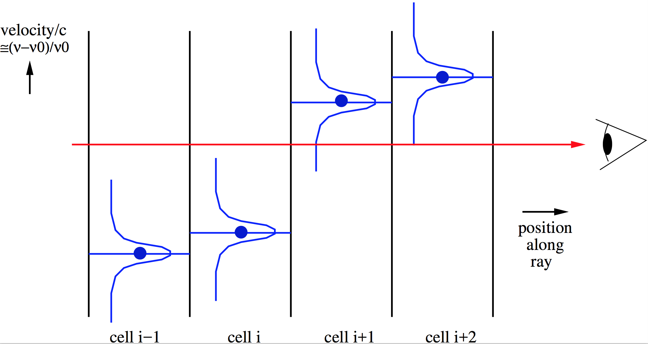
_images/line_doppjump.png — Fig. 7 Pictographic representation of the doppler jumping problem with ray-tracing through a model with strong cell-to-cell velocity differences.

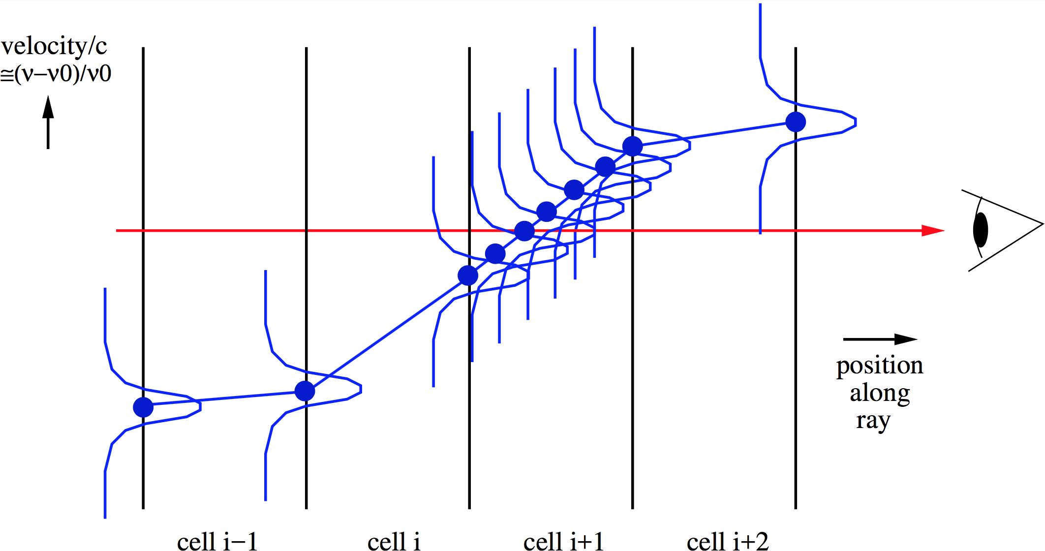
_images/line_doppcatch.png — Fig. 8 Right: Pictographic representation of the doppler catching method to prevent this problem: First of all, second order integration is done instead of first order. Secondly, the method automatically detects a possibly dangerous doppler jump and makes sub-steps to neatly integrate over the line that shifts in- and out of the wavelength channel of interest.

The problem is described in more detail in Section Heads-up: In reality wavelength are actually wavelength bands, and one possible solution is proposed there. But that solution does not always solve the problem.

RADMC-3D has a special method to catch situations like the above, and when it detects one, to make sub-steps in the integration of the formal transfer equation so that the smooth passing of the line through the wavelength-of-sight can be properly accounted for. Here this is called ‘doppler catching’, for lack of a better name. The technique was discussed in great detail in Pontoppidan et al. (2009, ApJ 704, 1482). The idea is that the method automatically tests if a line might ‘doppler jump’ over the current wavelength channel. If so, it will insert substeps in the integration at the location where this danger is present. See Fig. Fig. 8 for a pictographic representation of this method. Note that this method can only be used with the second order ray-tracing (see Section Second order ray-tracing (Important information!)); in fact, as soon as you switch the doppler catching on, RADMC-3D will automatically also switch on the second order ray-tracing.

To switch on doppler catching, you simply add the command-line option doppcatch to the image or spectrum command. For instance:

radmc3d spectrum iline 1 widthkms 10 doppcatch

(again: you do not need to add secondorder, because it is automatic when doppcatch is used).

The Doppler catching method will assure that the line is integrated over with small enough steps that it cannot accidently get jumped over. How fine these steps will be can be adjusted with the catch_doppler_resolution keyword in the radmc3d.inp file. The default value is 0.2, meaning that it will make the integration steps small enough that the doppler shift over each step is not more than 0.2 times the local intrinsic (thermal+microturbulent) line width. That is usually enough, but for some problems it might be important to ensure that smaller steps are taken. By adding a line:

catch_doppler_resolution = 0.05

to the radmc3d.inp file you will ensure that steps are small enough that the doppler shift is at most 0.05 times the local line width.

So why is doppler catching an option, i.e. why would this not be standard? The reason is that doppler catching requires second order integration, which requires RADMC-3D to first map all the cell-based quantities to the cell-corners. This requires extra memory, which for very large models can be problematic. It also requires more CPU time to calculate images/spectra with second order integration. So if you do not need it, i.e. if your velocity gradients are not very steep compared to the intrinsic line width, then it saves time and memory to not use doppler catching.

It is, however, important to realize that doppler catching is not the golden bullet. Even with doppler catching it might happen that some line flux is lost, but this time as a result of too low image resolution. This is less likely to happen in problems like ISM turbulence, but it is pretty likely to happen in models of rotating disks. Suppose we have a very thin local line width (i.e. low gas temperature and no microturbulence) in a rotating thin disk around a star. In a given velocity channel (i.e. at a given observer-frame frequency) a molecular line in the disk emits only in a very thin ‘ear-shaped’ ring or band in the image. The thinner the intrinsic line width, the thinner the band on the image. See Pontoppidan et al. (2009, ApJ 704, 1482) and Pavlyuchenkov et al. (2007, ApJ 669, 1262) for example. If the pixel-resolution of the image is smaller than that of this band, the image is simply underresolved. This has nothing to do with the doppler jumping problem, but can be equally devastating for the results if the user is unaware of this. There appears to be only one proper solution: assure that the pixel-resolution of the image is sufficiently fine for the problem at hand. This is easy to find out: The image would simply look terribly noisy if the resolution is insufficient. However, if you are not interested in the images, but only in the spectra, then some amount of noisiness in the image (i.e. marginally sufficient resolution) is OK, since the total flux is an integral over the entire image, smearing out much of the noise. It requires some experimentation, though.

Here are some additional issues to keep in mind:

The doppler catching method uses second order integration (see Section Second order ray-tracing (Important information!)), and therefore all the relevant quantities first have to be interpolated from the cell centers to the cell corners. Well inside the computational domain this amounts to linear interpolation. But at the edges of the domain it would require extra polation. In 1-D this is more easily illustrated, because there the cell corners are in fact cell interfaces. Cells \(i\) and \(i+1\) share cell interface \(i+1/2\). If we have \(N\) cells, i.e. cells \(i=1,\cdots,N\), then we have \(N+1\) interfaces, i.e. interfaces \(i=\tfrac{1}{2},\cdots,N+\tfrac{1}{2}\). To get physical quantities from the cell centers to cell interfaces \(i=\tfrac{3}{2},\cdots,N-\tfrac{1}{2}\) requires just interpolation. But to find the physical quantities at cell interfaces \(i=\tfrac{1}{2}\) and \(i=N+\tfrac{1}{2}\) one has to extrapolate or simply take the values at the cell centers \(i=1\) and \(i=N\). RADMC-3D does not do extrapolation but simply takes the average values of the nearest cells. Also the gas velocity is treated like this. This means that over the edge cells the gradient in the gas velocity tends to be (near) 0. Since for the doppler catching it is the gradient of the velocity that matters, this might yield some artifacts in the spectrum if the density in the border cells is high enough to produce substantial line emission. Avoiding this numerical artifact is relatively easy: One should then simply put the number density of the molecule in question to zero in the boundary cells.
If you are using RADMC-3D on a 3-D (M)HD model which has strong shocks in its domain, then one must be careful that (magneto-)hydrodynamic codes tend to smear out the shock a bit. This means that there will be some cells that have intermediate density and velocity in the smeared out region of the shock. This is unphysical, but an intrinsic numerical artifact of numerical hydrodynamics codes. This might, under some conditions, lead to unphysical signal in the spectrum, because there would be cells at densities, temperatures and velocities that would be in between the values at both sides of the shock and would, in reality, not be there. It is very difficult to avoid this problem, and even to find out if this problem is occurring and by how much. One must simply be very careful of models containing strong shocks and do lots of testing. One way to test is to use the doppler catching method and vary the doppler catching resolution (using the catch_doppler_resolution keyword in radmc3d.inp).
If using line transfer in spherical coordinates using doppler catching, the linear interpolation of the line shift between the beginning and the end of a segment may not always be enough to accurately prevent doppler jumps. This is because in addition to the physical gradient of gas velocity, the projected gas velocity along a ray changes also along the ray due to the geometry (the use of spherical coordinates). Example: a spherically symmetric radially outflowing wind with constant outward velocity \(v_r=`const. Although :math:`v_r\) is constant, the 3-D vector \(\vec v\) is not constant, since it always points outward. A ray through this wind will thus have a varying \(\vec n\cdot \vec v\) along the ray. In the cell where the ray reaches its closest approach to the origin of the coordinate system the \(\vec n\cdot \vec v\) will vary the strongest. This may be such a strong effect that it could affect the reliability of the code. As of version 0.41 of this code a method is in place to prevent this. It is switched on by default, but it can be switched off manually for testing purposes. See Section Second order integration in spherical coordinates: a subtle issue for details.

Background information: Calculation and storage of level populations

If RADMC-3D makes an image or a spectrum with molecular (or atomic) lines included, then the level populations of the molecules/atoms have to be computed. In the standard method of ray-tracing of images or spectra, these level populations are first calculated in each grid cell and stored in a global array. Then the raytracer will render the image or spectrum.

The storage of the level populations is a tricky matter, because if this is done in the obvious manner, it might require a huge amount of memory. This would then prevent us from making large scale models. For instance: if you have a molecule with 100 levels in a model with 256x256x256 \(\simeq 1.7\times 10^7\) cells, the global storage for the populations alone (with each number in double precision) would be roughly 100x8x256x256x256 \(\simeq\) 13 Gigabyte.

However, if you intend to make a spectrum in just 1 line, you do not need all these level populations. To stick to the above example, let us take the CO 1-0 line, which is then line 1 and which connects levels \(J=1\) and \(J=0\), which are levels 2 and 1 in the code (if you use the Leiden database CO data file). Once the populations have been computed, we only need to store the levels 1 and 2. This would then require 2x8x256x256x256 \(\simeq\) 0.26 Gigabyte, which would be much less memory-costly.

As of version 0.29 RADMC-3D automatically figures out which levels have to be stored in a global array, in order to be able to render the images or the spectrum properly. RADMC-3D will go through all the lines of all molecules and checks if they contribute to the wavelength(s), of the image(s) or the spectrum. Once it has assembled a list of ‘active’ lines, it will make a list of ‘active’ levels that belong to these lines. It will then declare this to be the ‘subset’ of levels for which the populations will be stored globally.

In other words: RADMC-3D now takes care of the memory-saving storage of the populations automatically.

How does RADMC-3D decide whether a line contributes to some wavelength \(\lambda\)? A line \(i\) with line center \(\lambda_i\) is considered to contribute to an image at wavelength \(\lambda\) if

\[| \lambda_i-\lambda | \le C_{\mathrm{margin}}\Delta\lambda_i\]

where \(\Delta\lambda_i\) is the line width (including all contributions) and \(C_{\mathrm{margin}}\) is a constant. By default

\[C_{\mathrm{margin}} = 12\]

But you can change this to another value, say 24, by adding in the radmc3d.inp file a line containing, e.g. lines_widthmargin = 24.

You can in fact get a dump of the level populations that have been computed and used for the image(s)/spectrum you created, by adding writepop on the command line. Example:

radmc3d spectrum iline 1 widthkms 10 writepop

This then creates (in addition to the spectrum) a file called (for our example of the CO molecule) levelpop_co.dat. Here is how you can read this data in Python:

from radmc3d_tools import simpleread
data = simpleread.read_levelpop()

The data object then contains data.pop and data.relpop, which are the level populations in \(1/cm^3\) and in normalized form.

If, for some reason, you want always all levels to be stored (and you can afford to do so with the size of your computer’s memory), you can make RADMC-3D do so by adding noautosubset as a keyword to the command line, or by adding lines_autosubset = 0 to the radmc3d.inp file. However, for other than code testing purposes, it seems unlikely you will wish to do this.

In case it is necessary: On-the-fly calculation of populations

There might be rare circumstances in which you do not want to have to store the level populations in a global array. For example: you are making a spectrum of the CO bandhead, in which case you have many tens of lines in a single spectrum. If your model contains 256x256x256 cells (see example in Section Background information: Calculation and storage of level populations) then this might easily require many Gigabytes of memory just to store the populations.

For the LTE, LVG and optically thin level population modes there is a way out: You can force RADMC-3D to compute the populations on-the-fly during the ray-tracing, which does not require a global storage of the level populations.

The way to do this is simple: Just make the lines_mode negative. So for on-the-fly LTE mode use lines_mode=-1, for on-the-fly user-defined populations mode use lines_mode=-2, for on-the-fly LVG mode use lines_mode=-3 and for on-the-fly optically thin populations use lines_mode=-4.

NOTE: The drawback of this method is that, under certain circumstances, it can slow down the code dramatically. This slow-down happens if you use e.g. second-order integration (Section Second order ray-tracing (Important information!)) and/or doppler catching (Section Preventing doppler jumps: The ‘doppler catching method’) together with non-trivial population solving methods like LVG. So please use the on-the-fly method only when you are forced to do so (for memory reasons).

For experts: Selecting a subset of lines and levels ‘manually’

As explained in Section Background information: Calculation and storage of level populations, RADMC-3D automatically makes a selection of levels for which it will allocate memory for the global level population storage.

If, for some reason, you wish to make this selection yourself ‘by hand’, this can also be done. However, please be informed that there are very few circumstances under which you may want to do this. The automatic subset selection of RADMC-3D is usually sufficient!

If you decided to really want to do this, here is how:

Switch off the automatic subset selection by adding noautosubset as a keyword to the command line, or by adding lines_autosubset = 0 to the radmc3d.inp file.
In the lines.inp file, for each molecule, modify the ‘0 0’ (the first two zeroes after ‘leiden’) in the way described below.

In Section INPUT: The line.inp file you can see that each molecule has a line like:

co   leiden   0  0  0

or so (here for the example of CO). In Section INPUT: The line.inp file we explained the meaning of the third number, but we did not explain the meaning of the first and second ones. These are meant for this subset selection. If we want to store only the first 10 levels of the CO molecule, then replace the above line with:

co   leiden   0  10  0

If you want to select specific levels (let us choose the ilevel=3 and ilevel=4 levels of the above example), then write:

co   leiden   1  2  0
3 4

The ‘1’ says that a list of levels follows, the ‘2’ says that two levels will be selected and the next line with ‘3’ and ‘4’ say that levels 3 and 4 should be selected.