More information about the gridding
We already discussed the various types of grids in Section The spatial grid, and the grid input file structure is described in Section INPUT (required): amr_grid.inp. In this chapter let us take a closer look at the gridding possibilities and things to take special care of.
Regular grids
A regular grid is called ‘grid style 0’ in RADMC-3D. It can be used in Cartesian coordinates as well as in spherical coordinates (Section Coordinate systems).
A regular grid, in our definition, is a multi-dimensional grid which is separable in \(x\), \(y\) and \(z\) (or in spherical coordinates in \(r\), \(\theta\) and \(\phi\)). You specify a 1-D monotonically increasing array of values \(x_1, x_2,\cdots,x_{\mathrm{nx+1}}\) which represent the cell walls in \(x-direction\). You do the same for the other directions: \(y_1, y_2,\cdots,y_{\mathrm{ny+1}}\) and \(z_1, z_2,\cdots,z_{\mathrm{nz+1}}\). The value of, say, \(x_2\) is the same for every position in \(y\) and \(z\): this is what we mean with ‘separable’.
In Cartesian coordinates RADMC-3D enforces perfectly cubic grid cells (i.e. linear grids). But that is only to make the image sub-pixeling easier (see Section The solution: recursive sub-pixeling). For spherical grids this is not enforced, and in fact it is strongly encouraged to use non-linear grids in spherical coordinates. Please read Section Separable grid refinement in spherical coordinates (important!) if you use spherical coordinates!
In a regular grid you specify the grids in each direction separately. For instance, the x-grid is given by specifying the cell walls in x-direction. If we have, say, 10 cells in x-direction, we must specify 11 cell wall positions. For instance: \(x_i=\{-5,-4,-3,-2,-1,0,1,2,3,4,5\}\). For the \(y\)-direction and \(z\)-direction likewise. Fig. Fig. 21 shows an example of a 2-D regular grid of 4x3 cells.

Fig. 21 Example of a regular 2-D grid with nx=4 and ny=3.
In Cartesian coordinates we typically define our model in full 3-D. However, if your problem has translational symmetries, you might also want to consider the 1-D plane-parallel mode (see Section 1-D Plane-parallel models).
In full 3-D Cartesian coordinates the cell sizes must be perfectly cubical, i.e. the spacing in each direction must be the same. If you need a finer grid in some location, you can use the AMR capabilities discussed below.
In spherical coordinates you can choose between 1-D spherically symmetric models, 2-D axisymmetric models or fully 3-D models. In spherical coordinates you do not have restrictions to the cell geometry or grid spacing. You can choose any set of numbers \(r_1,\cdots,r_{\mathrm{nr}}\) as radial grid, as long as this set of numbers is larger than 0 and monotonically increasing. The same is true for the \(\theta\)-grid and the \(\phi\)-grid.
The precise way how to set up a regular grid using the amr_grid.inp file is
described in Section Regular grid. The input of any spatial
variables (such as e.g. the dust density) uses the sequence of grid cells in
the same order as the cells are specified in that amr_grid.inp file.
For input and output data to file, for stuff on a regular grid, the order of nested loops over coordinates would be:
do iz=1,amr_grid_nz
   do iy=1,amr_grid_ny
      do ix=1,amr_grid_nx
         << read or write your data >>
      enddo
   enddo
enddo
For spherical coordinates we have the following association: \(x\rightarrow r\), \(y\rightarrow \theta\), \(z\rightarrow \phi\).
Separable grid refinement in spherical coordinates (important!)
Spherical coordinates are a very powerful way of dealing with centrally-concentrated problems. For instance, collapsing protostellar cores, protoplanetary disks, disk galaxies, dust tori around active galactic nuclei, accretion disks around compact objects, etc. In other words: problems in which a single central body dominates the problem, and material at all distances from the central body matters. For example a disk around a young star goes all the way from 0.01 AU out to 1000 AU, covering 5 orders of magnitude in radius. Spherical coordinates are the easiest way of dealing with such a huge radial dynamic range: you simply make a radial grid, where the grid spacing \(r_{i+1}-r_i\) scales roughly with \(r_i\).
This is called a logarithmic radial grid. This is a grid whith a spacing in which \((r_{i+1}-r_i)/r_i\) is constant with \(r\). In this way you assure that you have always the right spatial resolution in \(r\) at each radius. In spherical coordinates it is highly recomended to use such a log spacing. But you can also refine the \(r\) grid even more (in addition to the log-spacing). This is also strongly recommended near the inner edge of a circumstellar shell, for instance. Or at the inner dust rim of a disk. There you must refine the \(r\) grid (by simply making the spacing smaller as you approach the inner edge from the outside) to assure that the first few cells are optically thin and that there is a gradual transition from optically thin to optically thick as you go outward. This is particularly important for, for instance, the inner rim of a dusty disk.
In spherical coordinates you can vary the spacing in \(r\), \(\theta\) and \(\phi\) completely freely. That means: you could have for instance \(r\) to be spaced as \(1.00, 1.01, 1.03, 1.05, 1.1, 1.2, 1.35, \cdots\). There is no restriction, as long as the coordinate points are monotonically increasing. In Figs Fig. 22 and Fig. 23 this is illustrated.
Note that in addition to separable refinement, also AMR refinement is possible in spherical coordinates. See Section Oct-tree Adaptive Mesh Refinement.
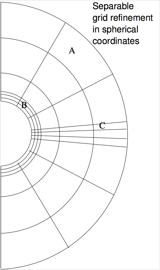
Fig. 22 Example of a spherical 2-D grid in which the radial and \(\theta\) grids are refined in a ‘separable’ way. In radial direction the inner cells are refined (‘B’ in the right figure) and in \(\theta\) direction the cells near the equatorial plane are refined (‘C’ in the right figure). This kind of grid refinement does not require oct-tree AMR: the grid remains separable. For models in which the inner grid edge is also the inner model edge (e.g. a simple model of a protoplanetary disk with a sharp inner cut-off) this kind of separable grid refinement in \(R\)-direction may be essential to avoid problems with optically thick inner cells (see e.g. Fig. Fig. 30 for an example of what could go wrong if you do not do this). Separable grid refinement in \(\Theta\)-direction is typically important for protoplanetary disk models, where the midplane and surface layers of the disk need to have sufficient resolution, but any possible surrounding spherical nebula may not.
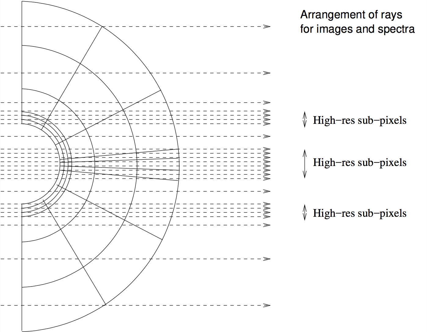
Fig. 23 When making an image, RADMC-3D will automatically make ‘sub-pixels’ to ensure that all structure of the model as projected on the sky of the observer are spatially resolved. Extreme grid refinement leads thus to extreme sub-pixeling. See Section Recursive sub-pixeling in spherical coordinates for details, and ways to prevent excessive sub-pixeling when this is not necessary.
For models of accretion disks it can, for instance, be useful to make sure that there are more grid points of \(\theta\) near the equatorial plane \(\theta=\pi/2\). So the grid spacing between \(\theta=0.0\) and \(\theta=1.0\) may be very coarse while between \(\theta=1.0\) and \(\theta=\pi/2\) you may put a finer grid. All of this ‘grid refinement’ can be done without the ‘AMR’ refinement technique: this is the ‘separable’ grid refinement, because you can do this separately for \(r\), for \(\theta\) and for \(\phi\).
Sometimes, however, separable refinement may not help you to refine the grid where necessary. For instance: if you model a disk with a planet in the disk, then you may need to refine the grid around the planet. You could refine the grid in principle in a separable way, but you would then have a large redundancy in cells that are refined by far away from the planet. Or if you have a disk with an inner rim that is not exactly at \(r=r_{\mathrm{rim}}\), but is a rounded-off rim. In these cases you need refinement exactly located at the region of interest. For that you need the ‘AMR’ refinement (Sections Oct-tree Adaptive Mesh Refinement and Layered Adaptive Mesh Refinement).
Important note: When using strong refinement in one of the coordinates \(r\), \(\theta\) or \(\phi\), image-rendering and spectrum-rendering can become very slow, because of the excessive sub-pixeling this causes. There are ways to limit the sub-pixeling for those cases. See the Section on sub-pixeling in spherical coordinate: Section Recursive sub-pixeling in spherical coordinates.
Oct-tree Adaptive Mesh Refinement
An oct-tree refinened grid is called ‘grid style 1’ in RADMC-3D. It can be used in Cartesian coordinates as well as in spherical coordinates (Section Coordinate systems).
You start from a normal regular base grid (see Section Regular grids), possibly even with ‘separable refinement’ (see Section Separable grid refinement in spherical coordinates (important!)). You can then split some of the cells into 2x2x2 subcells (or more precisely: in 1-D 2 subcells, in 2-D 2x2 subcells and in 3-D 2x2x2 subcells). If necessary, each of these 2x2x2 subcells can also be split into further subcells. This can be repeated as many times as you wish until the desired grid refinement level is reached. Each refinement step refines the grid by a factor of 2 in linear dimension, which means in 3-D a factor of 8 in volume. In this way you get, for each refined cell of the base grid, a tree of refinement. The base grid can have any size, as long as the number of cells in each direction is an even number. For instance, you can have a 6x4 base grid in 2-D, and refine cell (1,2) by one level, so that this cell splits into 2x2 subcells.
Note that it is important to set which dimensions are ‘active’ and which are ‘non-active’. For instance, if you have a 1-D model with 100 cells and you tell RADMC-3D (see Section Oct-tree-style AMR grid) to make a base grid of 100x1x1 cells, but you still keep all three dimensions ‘active’ (see Section Oct-tree-style AMR grid), then a refinement of cell 1 (which is actually cell (1,1,1)) will split that cell into 2x2x2 subcells, i.e. it will also refine in y and z direction. Only if you explicitly switch the y and z dimensions off the AMR will split it into just 2 subcells.
Oct-tree mesh refinement is very powerful, because it allows you to refine the grid exactly there where you need it. And because we start from a regular base grid like the grid specified in Section Regular grids, we can start designing our model on a regular base grid, and then refine where needed. See Fig. Fig. 24.
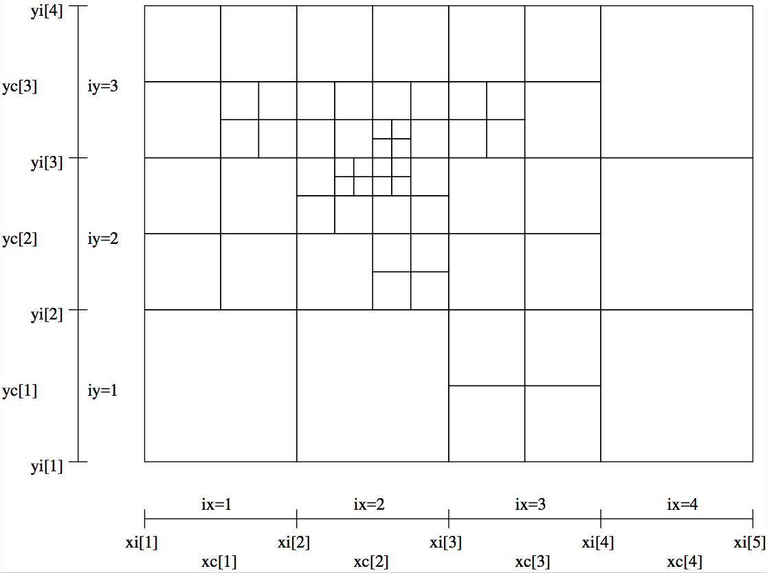
Fig. 24 Example of a 2-D grid with oct-tree refinement. The base grid has nx=4
and ny=3. Three levels of refinement are added to this base grid.
The AMR stand for ‘Adaptive Mesh Refinement’, which may suggest that RADMC-3D will refine internally. At the moment this is not yet the case. The ‘adaptive’ aspect is left to the user: he/she will have to ‘adapt’ the grid such that it is sufficiently refinened where it is needed. In the future we may allow on-the-fly adaption of the grid, but that is not yet possible now.
One problem with oct-tree AMR is that it is difficult to handle such grids in
external plotting programs, or even in programs that set up the grid. While it
is highly flexible, it is not very user-friendly. Typically you may use this
oct-tree refinement either because you import data from a hydrodynamics code
that works with oct-tree refinement (e.g. FLASH, RAMSES), or when you
internally refine the grid using the userdef_module.f90 (see Chapter
Modifying RADMC-3D: Internal setup and user-specified radiative processes). In the former case you are anyway forced to manage
the complexities of AMR, while in the latter case you can make use of the AMR
modules of RADMC-3D internally to handle them. But if you do not need to full
flexibility of oct-tree refinement and want to use a simpler kind of refinement,
then you can use RADMC-3D’s alternative refinement mode: the layer-style AMR
described in Section Layered Adaptive Mesh Refinement below.
The precise way how to set up such an oct-tree grid using the amr_grid.inp
file is described in Section Oct-tree-style AMR grid. The input of any
spatial variables (such as e.g. the dust density) uses the sequence of grid
cells in the same order as the cells are specified in that amr_grid.inp
file.
Layered Adaptive Mesh Refinement
A layer-style refinened grid is called ‘grid style 10’ in RADMC-3D. It can be used in Cartesian coordinates as well as in spherical coordinates (Section Coordinate systems).
This is an alternative to the full-fledged oct-tree refinement of Section Oct-tree Adaptive Mesh Refinement. The main advantage of the layer-style refinement is that it is far easier to handle by the human brain, and thus easier for model setup and the analysis of the results.
The idea here is that you start again with a regular grid (like that of Section Regular grids), but you can now specify a rectangular region which you want to refine by a factor of 2. The way you do this is by choosing the starting indices of the rectangle and specifying the size of the rectangle by setting the number of cells in each direction from that starting point onward. For instance, setting the starting point at (2,3,1) and the size at (1,1,1) will simply refine just cell (2,3,1) of the base grid into a set of 2x2x2 sub-cells. But setting the starting point at (2,3,1) and the size at (2,2,2) will split cells (2,3,1), (3,3,1), (2,4,1), (3,4,1), (2,3,2), (3,3,2), (2,4,2) and (3,4,2) each into 2x2x2 subcells. This in fact is handled as a 4x4x4 regular sub-grid patch. And setting the starting point at (2,3,1) and the size at (4,6,8) will make an entire regular sub-grid patch of 8x12x16 cells. Such a sub-grid patch is called a layer.
The nice thing of these layers is that each layer (i.e. subgrid patch) is handled as a regular sub-grid. The base grid is layer number 0, and the first layer is layer number 1, etc. Each layer (including the base grid) can contain multiple sub-layers. The only restriction is that each layer fits entirely inside its parent layer, and layers with the same parent layer should not overlap. Each layer can thus have one or more sub-layers, each of which can again be divided into sub-layers. This builds a tree structure, with the base layer as the trunk of the tree (this is contrary to the oct-tree structure, where each base grid cell forms the trunk of its own tree). In Fig. Fig. 25 an example is shown of two layers with the same parent (= layer 0 = base grid), while in Fig. Fig. 26 an example is shown of two nested layers.
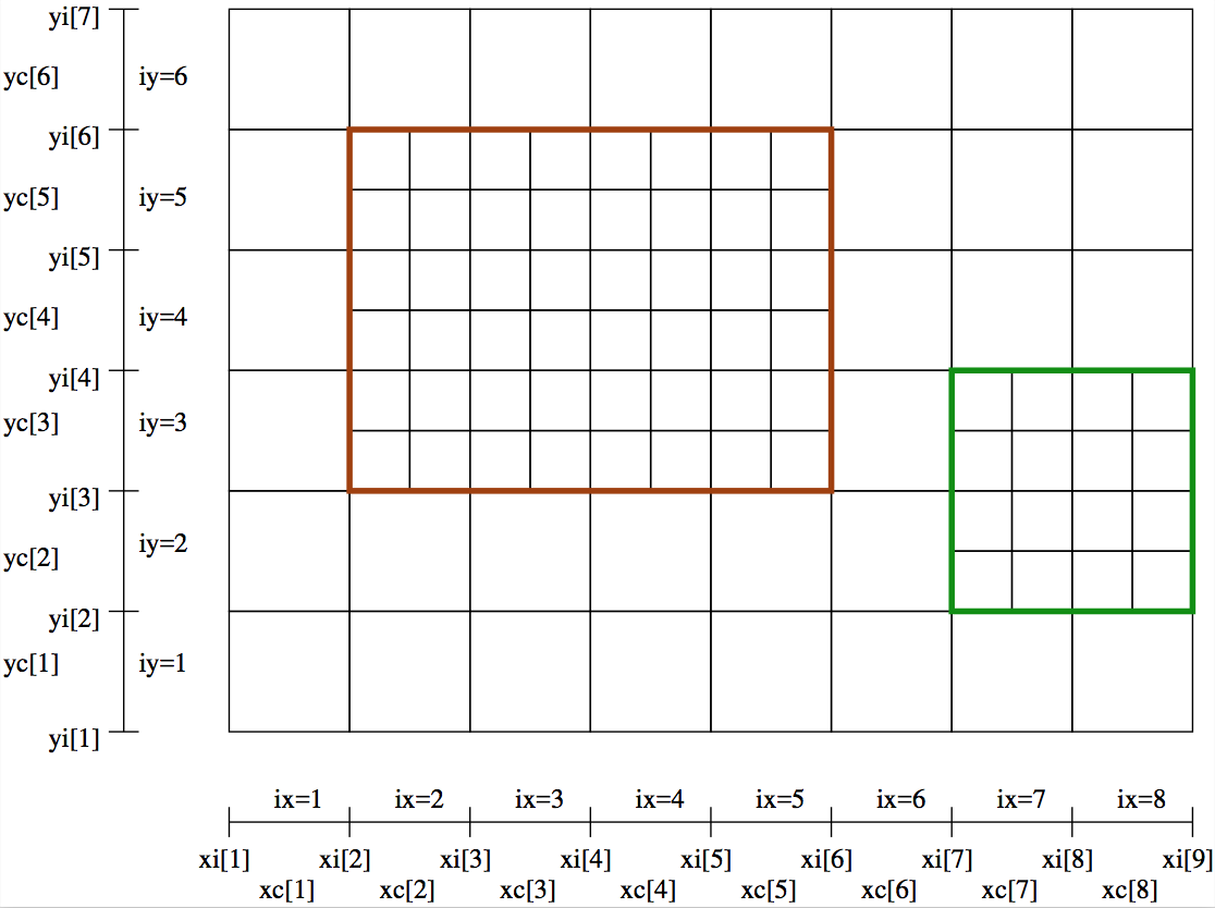
Fig. 25 Example of a 2-D base grid with nx=4 and ny=3, with two
AMR-layers added to it. This example has just one level of refinement, as
the two layers (brown and green) are on the same level (they have the same
parent layer = layer 0).
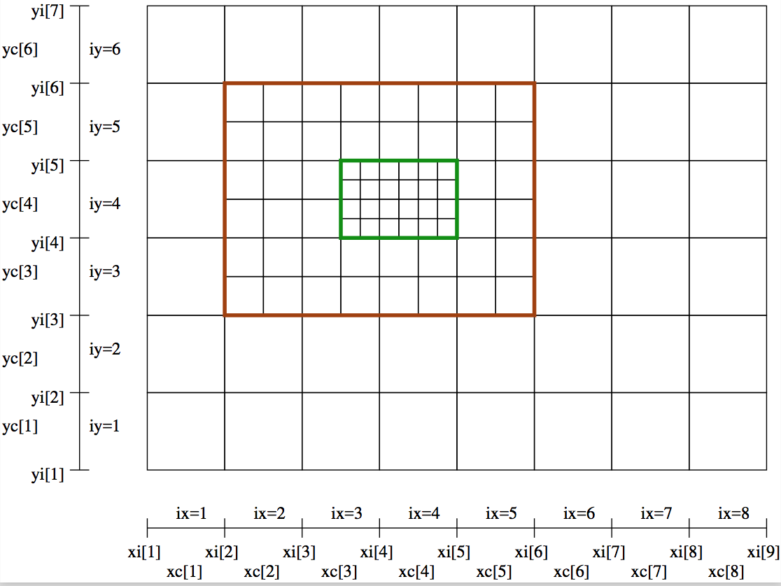
Fig. 26 Example of a 2-D base grid with nx=4 and ny=3, with two nested
AMR-layers added to it. This example has two levels of refinement, as layer
1 (brown) is the parent of layer 2 (green).
If you now want to specify data on this grid, then you simply specify it on
each layer separately, as if each layer is a separate entity. Each layer is
treated as a regular grid, irrespective of whether it contains sub-layers
or not. So if we have a base grid of 4x4x4 grid cells containing two layers:
one starting at (1,1,1) and having (2,2,2) size and another starting at
(3,3,3) and having (1,1,2) size, then we first specify the data on the
\(4^3=64\) base grid, then on the \((2\times 2)^3=64\) grid cells of the first
layer and then on the 2x2x4=16 cells of the second layer. Each of these
three layers are regular grids, and the data is inputted/outputted in
the same way as if these are normal regular grids (see Section
Regular grids). But instead of just one such regular grid, now
the data file (e.g. dust_density.inp) will contain three
successive lists of numbers, the first for the base grid, the second for
the first layer and the last for the second layer. You may realize at this
point that this will introduce a redundancy. See Subsection
On the ‘successively regular’ kind of data storage, and its slight redundancy for a discussion of this redundancy.
The precise way how to set up such an oct-tree grid using the amr_grid.inp
file is described in Section Layer-style AMR grid. The input of any
spatial variables (such as e.g. the dust density) uses the sequence of grid
cells in the same order as the cells are specified in that amr_grid.inp
file.
On the ‘successively regular’ kind of data storage, and its slight redundancy
With the layered grid refinement style there will be redundant data in the
data files (such as e.g. the dust_density.inp file. Each layer is a regular
(sub-)grid and the data will be specified in each of these grid cells of that
regular (sub-)grid. If then some of these cells are overwritten by a
higher-level layer, these data are then redundant. We could of course have
insistent that only the data in those cells that are not refined by a layer
should be written to (or read from) the data files. But this would require quite
some clever programming on the part of the user to a-priori find out where the
layers are and therefore which cells should be skipped. We have decided that it
is far easier to just insist that each layer (including the base grid, which is
layer number 0) is simply written to the data file as a regular block of
data. The fact that some of this data will be not used (because they reside in
cells that are refined) means that we write more data to file than really exists
in the model. This makes the files larger than strictly necessary, but it makes
the data structure by far easier. Example: suppose you have a base grid of 8x8x8
cells and you replace the inner 4x4x4 cells with a layer of 8x8x8 cells (each
cell being half the size of the original cells). Then you will have for
instance a dust_density.inp file containing 1024 values of the density:
\(8^3\)=512 values for the base grid and again \(8^3\)=512 values for
the refinement layer. Of the first \(8^3\)=512 values \(4^3\)=64 values
are ignored (they could have any value as they will not be used). The file is
thus 64 values larger than strictly necessary, which is a redundancy of
64/1024=0.0625. If you would have used the oct-tree refinement style for making
exactly the same grid, you would have only 1024-64=960 values in your file,
making the file 6.25% smaller. But since 6.25% is just a very small
difference, we decided that this is not a major problem and the simplicity of
our ‘successively regular’ kind of data format is more of an advantage than the
6.25% redundance is a disadvantage.
Unstructured grids
In a future version of RADMC-3D we will include unstructured gridding as a possibility. But at this moment such a gridding is not yet implemented.
1-D Plane-parallel models
Sometimes it can be useful to make simple 1-D plane parallel models, for instance if you want to make a simple 1-D model of a stellar atmosphere. RADMC-3D is, however, by nature a 3-D code. But as of version 0.31 it features a genuine 1-D plane-parallel mode as well. This coordinate type has the number 10. In this mode the \(x\)- and \(y\)-coordinates are the in-plane coordinates, while the \(z\)-coordinate is the 1-D coordinate. We thus have a 1-D grid in the \(z\)-coordinate, but no grid in \(x\)- or \(y\)-directions.
You can make a 1-D plane-parallel model by setting some settings in the
amr_grid.inp file. Please consult Section INPUT (required): amr_grid.inp for the
format of this file. The changes/settings you have to do are (see example
below): (1) set the coordinate type number to 10, (2) set the \(x\) and
\(y\) dimensions to non-active and (3) setting the cell interfaces in
\(x\) to -1d90, +1d90, and likewise for \(y\). Here is then how it
looks:
1                                     <=== Format number = 1
0                                     <=== Grid style (0=regular grid)
10                                    <=== Coordinate type (10=plane-parallel)
0                                     <=== (obsolete)
0  0  1                               <=== x and y are non-active, z is active
1  1  100                             <=== x and y are 1 cell, in z we have 100 cells
-1e90 1e90                            <=== cell walls in x are at "infinity"
-1e90 1e90                            <=== cell walls in y are at "infinity"
zi[1]        zi[2]        zi[3]       ........  zi[nz+1]
The other input files are for the rest as usual, as in the 3-D case.
You can now make your 1-D model as usual. For 1-D plane-parallel problems it is often useful to put a thermal boundary at the bottom of the model. For instance, if the model is a stellar atmosphere, you may want to cap the grid from below with some given temperature. See Section Thermal boundaries in Cartesian coordinates for details on how to set up thermal boundaries.
In the 1-D plane-parallel mode some things work a bit different than in the “normal” 3-D mode:
Images are by default 1x1 pixels, because in a plane-parallel case it is useless to have multiple pixels.
Spectra cannot be made, because “spectrum” is (in RADMC-3D ‘language’) the flux as a function of frequency as seen at a very large distance of the object, so that the object is in the “far field”. Since the concept of “far-field” is no longer meaningful in a plane-parallel case, it is better to make frequency-dependent 1x1 pixel images. This gives you the frequence-dependent intensity, which is all you should need.
Stars are not allowed, as they have truly 3-D positions, which is inconsistent with the plane-parallel assumption.
But for the rest, most stuff works similarly to the 3-D version. For instance, you can compute dust temperatures with
radmc3d mctherm
as usual.
Making a spectrum of the 1-D plane-parallel atmosphere
As mentioned above, the ‘normal’ 3-D way of making a spectrum of the 1-D plane-parallel atmosphere is not possible, because formally the atmosphere is infinitely extended. Instead you can obtain a spectrum in the form of an intensity (\(\mathrm{erg}\,\mathrm{s}^{-1}\,\mathrm{cm}^{-2}\,\mathrm{Hz}^{-1}\,\mathrm{ster}^{-1}\)) as a function of wavelength. To do this you ask RADMC-3D to make a multi-wavelength image of the atmosphere under a certain inclination (inclination 0 meaning face-on), e.g.:
radmc3d image allwl incl 70
This make an SED at \(\lambda=10\,\mu\)m for the observer seeing the
atmosphere at an inclination of 70 degrees. This produces a file image.out,
described in Section OUTPUT: image.out or image_****.out. The image is, in fact, a 1x1 pixel
multi-wavelength image. The allwl (which stands for ‘all wavelengths’) means
that the spectral points are the same as those in the wavelength_micron.inp
file (see Section INPUT (required): wavelength_micron.inp). You can also specify the wavelengths
in a different way, e.g.:
radmc3d image lambdarange 5 20 nlam 10
In fact, see Section Making multi-wavelength images and Section Specifying custom-made sets of wavelength points for the camera for details.
In 1-D plane-parallel: no star, but incident parallel flux beams
In 1-D plane-parallel geometry it is impossible to include meaningful stars as
sources of photons. This is not a technical issue, but a mathematical truth: a
point in 1-D is in reality a plane in 3-D. As a replacement RADMC-3D offers
(only in 1-D plane-parallel geometry) the possibility of illuminating the 1-D
atmosphere from above with a flux, incident onto the atmosphere in a prescribed
angle. This allows you to model, e.g., the Earth’s atmosphere being illuminated
by the sun at a given time of the day. This is done by providing an ascii file
called illum.inp which has the following form (similar, but not identical,
to the stars.inp file, see Section INPUT (mostly required): stars.inp):
iformat                           <=== Put this to 2 !
nillum     nlam
theta[1]      phi[1]
  .             .
  .             .
theta[nillum] phi[nillum]
lambda[1]
  .
  .
lambda[nlam]
flux[1,illum=1]
  .
  .
flux[nlam,illum=1]
flux[1,illum=2]
  .
  .
flux[nlam,illum=2]
  .
  .
  .
  .
flux[nlam,illum=nstar]
Here nillum is the number of illuminating beams you want to
specify. Normally this is 1, unless you have, e.g., a planet around a double
star. The theta is the angle (in degrees) under which the beam impinges onto
the atmosphere. If you have theta=0, then the flux points vertically
downward (sun at zenith). If you have theta=89, then the flux points
almost parallel to the atmosphere (sunset). It is not allowed to put theta=90.
You can, if you wish, also put the source behind the slab, i.e. theta>90. Please note, however, that if you compute the spectrum of the
plane-parallel atmosphere the direct flux from these illumination beams does not
get picked up in the spectrum.
Similarity and difference between 1-D spherical and 1-D plane-parallel
Note that this 1-D plane-parallel mode is only available in \(z\)-direction, and only for cartesian coordinates! For spherical coordinates, a simple switch to 1-D yields spherically symmetric 1-D radiative transfer, which is, however, geometrically distinct from 1-D plane-parallel radiative transfer. However, you can also use a 1-D spherically symmetric setup to ‘emulate’ 1-D plane parallel problems: You can make, for instance, a radial grid in which \(r_{\mathrm{nr}}/r_1-1\ll 1\). An example: \(r=\{10000.0\), \(10000.1\), \(10000.2\), \(\cdots,\) \(10001.0\}\). This is not perfectly plane-parallel, but sufficiently much so that the difference is presumably indiscernable. The spectrum is then automatically that of the entire large sphere, but by dividing it by the surface area, you can recalculate the local flux. In fact, since a plane-parallel model usually is meant to approximate a tiny part of a large sphere, this mode is presumably even more realistic than a truly 1-D plane-parallel model.
Thermal boundaries in Cartesian coordinates
By default all boundaries of the computational domain are open, in the sense
that photons can move out freely. The only photons that move into the domain
from the outside are those from the interstellar radiation field (see Section
The interstellar radiation field: external source of energy) and from any stars that are located outside of the
computational domain (see Section INPUT (mostly required): stars.inp). For some purposes it might,
however, be useful to have one or more of the six boundaries in 3-D to be
closed. RADMC-3D offers the possibility, in cartesian coordinates, to convert
the boundaries (each of the six separately) to a thermal boundary, i.e. a
blackbody emitter at some user-secified temperature. If you want that the left
X-boundary is a thermal wall at T=100 Kelvin, then you add the following line to
the radmc3d.inp file:
thermal_boundary_xl = 100
and similarly for xr (right X-boundary), yl, yr, zl and/or zr. You can set this
for each boundary separately, and particularly you can choose to set just one or
just two of the boundaries to thermal boundaries. Note that setting
thermal_boundary_xl=0 is equivalent to switching off the thermal boundary.
Note that if you now make an image of the box, the ray-tracer will show you still the inside of the box, through any possible thermal boundary. In other words: for the imaging or spectra these thermal boundaries are opaque for radiation entering the grid, while they are transparent for radiation exiting the grid. In other words, we see the blackbody emission from the backside walls, but not of the frontside walls. In this way we can have a look inside the box in spite of the thermal walls.