Tips, tricks and problem hunting
Tips and tricks
RADMC-3D is a large software package, and the user will in all likelihood not understand all its internal workings. In this section we will discuss some issues that might be useful to know when you do modeling.
Things that can drastically slow down ray-tracing:
When you create images or spectra,
radmc3dwill perform a ray-tracing calculation. You may notice that sometimes this can be very fast, but for other problems it can be very slow. This is because, depending on which physics is switched on, different ray-tracing strategies must be followed. For instance, if you use a dust opacity without scattering opacity (or if you switch dust scattering off by settingscattering_mode_maxto 0 in theradmc3d.inpfile), and you make dust continuum images, or make SEDs, this may go very rapidly: less than a minute on a modern computer for grids of 256x256x256. However, when you include scattering, it may go slower. Why is that? That is because at each wavelengthradmc3dwill now have to make a quick Monte Carlo scattering model to compute the dust scattering source function. This costs time. And it will cost more time if you havenphot_scatset to a high value in theradmc3d.inpfile, although it will create better images. Furthermore, if you also include gas lines using the simple LTE or simple LVG methods, then things become even slower, because each wavelength channel image is done after each other, and each time all the populations of the molecular levels have to be re-computed. If dust scattering would be switched off (which is for some wavelength domains presumably not a bad approximation; in particular for the millimeter domain), then no scattering Monte Carlo runs have to be done for each wavelength. Then the code can ray-trace all wavelength simultaneously: each ray is traced only once, for all wavelength simultaneously. Then the LTE/LVG level populations have to be computed only once at each location along the ray. So if you use dust and lines simultaneously, it can be advantageous for speed if you can afford to switch off the dust scattering, for instance, if you model sub-millimeter lines in regions with dust grains smaller than 10 micron or so. If you must include scattering, but your model is not so big that you may get memory limitation problems, then you may also try the fast LTE or fast LVG modes: in those modes the level populations are pre-computed before the ray-tracing starts, which saves time. But that may require much memory.
Bug hunting
Although we of course hope that radmc3d will not run into
troubles or crash, it is nevertheless possible that it will. There are
several ways by which one can hunt for bugs, and we list here a few
obvious ones:
In principle the
Makefileshould make sure that all dependencies of all modules are correct, so that the most dependent modules are compiled last. But during the further development of the code perhaps this may be not 100% guaranteed. So try domakecleanfollowed bymake(ormakeinstall) to assure a clean make.In the
Makefileyou can add (or uncomment) the lineBCHECK=-fbounds-check, if you usegfortran. Find the array boundary check switch on your own compiler if it is notgfortran.Make sure that in the
main.f90code the variabledebug_check_allis set to 1. This will do some on-the-fly checks in the code.
Some tips for avoiding troubles and for making good models
Here is a set of tips that we recommend you to follow, in order to avoid troubles with the code and to make sure that the models you make are OK. This list is far from complete! It will be updated as we continue to develop the code.
Make a separate directory for each model. This avoids confusion with the many input and output files from the models.
When experimenting: regularly keep models that work, and continue experimenting with a fresh model directory. If things go wrong later, you can always fall back on an older model that did work well.
Keep model directories within a parent directory of the code, just like it is currently organized. This ensures that each model is always associated to the version of the code for which it was developed. If you update to a new version of the code, it is recommended to simply copy the models you want to continue with to the new code directory (and edit the
SRCvariable in theMakefileif you use the techniques described in Section Making special-purpose modified versions of RADMC-3D (optional) and Chapter Modifying RADMC-3D: Internal setup and user-specified radiative processes).If you make a new model, try to start with as clean a directory as possible. This avoids that you accidently have a old files hanging around, their presence of which may cause troubles in your new model. So if you make a model update, make a new directory and then copy only the files that are necesary (for instance,
problem_setup.py,dustkappa_silicate.inp,Makefileand other necessary files). One way of doing this easily is to write a little perl script or csh script that does this for you.In the example model directories there is always a
Makefilepresent, even if no local*.f90files are present. The idea is that by typing {small make cleanall} you can safely clean up the model directory and restore it to pre-model status. This can be useful for safely cleaning model directories so that only the model setup files remain there. It may save enormous amounts of disk space. But of course, it means that if you revisit the model later, you would need to redo the Monte Carlo simulations again, for instance. It is a matter of choice between speed of access to results on the one hand and disk space on the other hand.If you use LVG or escape probability to compute the level populations of molecules, please be aware that you must include all levels that could be populated, not only the levels belonging to the line you are interested in.
Careful: Things that might go wrong
In principle RADMC-3D should be fine-tuned such that it produced reliable results in most circumstances. But radiative transfer modeling, like all kinds of modeling, is not an entirely trivial issue. Extreme circumstances can lead to wrong results, if the user is not careful in doing various sanity checks. This section gives some tips that you, the user, may wish to do to check that the results are ok. This is not an exhaustive list! So please remain creative yourself in coming up with good tests and checks.
Too low number of photon packages for thermal Monte Carlo
If the number of photon packages for the thermal Monte Carlo simulation (Section The thermal Monte Carlo simulation: computing the dust temperature) is too low, the dust temperatures are going to be very noisy. Some cells may even have temperature zero. This may not only lead to noisy images and spectra, but also simply wrong results. However, deep inside optically thick clouds (or protoplanetary disks) it will be hard to avoid this problem. Since those regions are very deep below the \(\tau=1\) surface, it might not be always too critical in that case. A bit of experimenting might be necessary.
Too low number of photon packages for scattering
When making images or spectra in which dust scattering is important, the scattered light emissivity is computed by a quick Monte Carlo simulation before the ray-tracing (see Section Scattered light in images and spectra: The ‘Scattering Monte Carlo’ computation). This requires the setting of the number of photon packages used for this (the variable
nphot_scatfor images and equivalentlynphot_specfor spectra, both can be set in theradmc3d.inpfile). If you see too much ‘noise’ in your scattering image, you can improve this by settingnphot_scatto a larger value (default = 100000). If your spectrum contains too much noise, try settingnphot_specto a larger value (default = 10000).Too optically thick cells at the surface or inner edge
You may want to experiment with grid resolution and refinement. Strictly speaking the transition from optically thin to optically thick, as seen both by the radiation entering the object and by the observer, has to occur over more than one cell. That is for very optically thick models, one may need to introduce grid refinement in various regions. As an example: an optically thick protoplanetary disk may have an extremely sharp thin-thick transition near the inner edge. To get the spectra and images right, it is important that these regions are resolved by the grid (note: once well inside the optically thick interior, it is no longer necessary to resolve individual optical mean free paths, thankfully). It should be said that in practice it is often impossible to do this in full strictness. But you may want to at least experiment a bit with refining the grid (using either ‘separable refinement’, see Section Separable grid refinement in spherical coordinates (important!), or AMR refinement, see Section Oct-tree-style AMR grid). An example how wrong things can go at the inner edge of a protoplanetary disk, if the inner cells are not assured to be optically thin through grid refinement (and possibly additionally a bit of smoothing of the density profile too) is given in Fig. Fig. 30.
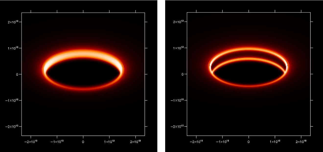
Fig. 30 Example of what can go wrong with radiative transfer if the inner cells of a model are optically thick (i.e.if no grid refinement is used, see Section Separable grid refinement in spherical coordinates (important!)). Shown here are scattered light images at \(\lambda=0.7\mu`m wavelength of the inner rim of a protoplanetary disk, but with the star removed with an ideal choronograph. The color scale is linear. The radial grid is taken to be logarithmically spaced with :math:\)Delta R/R=0.04`. Left image: the inner cells are marginally optically thin \(\Delta\tau\simeq 1\), creating a bright inner ring, as is expected. Right image: ten times higher optical depth, making the inner cells optically thick with roughly \(\Delta\tau\simeq 10\), resulting in a wrong image in which the emission near the midplane is strongly reduced. The reason for that is that the scattering source function, due to photons scattering at the inner 10% of the inner cell, is diluted over the entire cell, making the scattered light brighness 10x lower than it should be.
Model does not fit onto the grid (or onto the refined part of the grid)
The grid must be large enough to contain the entire \(\tau_\lambda=1\) surface of a model at all relevant wavelengths. If you use grid refinement, the same is true for the \(\tau_\lambda=1\) surface being within the refinened part of the grid. This is not trivial! If you, for instance, import a 3-D hydrodynamic model into RADMC-3D, then it is a common problem that the \(\tau_\lambda=1\) surface ‘wants’ to be outside of the grid (or outside of the higher-resolution part of the \(\theta\)-grid if you use separable grid refinement: see Fig. fig-spher-sep-ref). For example: if you make a * hydrodynamic* model of a protoplanetary disk in \(R\), \(\Theta\) and \(\Phi\) coordinates, you typically want to model only the lower 2 pressure scale heights of the disk, since that contains 99.5% of the mass of the disk. However, for radiative transfer this may not be enough, since if the disk has an optical depth of \(\tau=10^3\), the optically thin surface layer is less than \(0.1\%\) of the disk mass, meaning that you need to model the lower 3 (not 2!) pressure scale heights. Simply inserting the hydrodynamics model with the first 2 scale heights would lead to an artifical cut-off of the disk. In other words, the real \(\tau_\lambda=1\) surface ‘wants’ to be outside of the grid (or outside of the refined part of the grid). This leads to wrong results.
Common technical problems and how to fix them
When using a complex code such as RADMC-3D there are many ways you might encounter a problem. Here is a list of common issues and tips how to fix them.
After updating RADMC-3D to a new version, some setups don’t work anymore.
This problem can be due to several things:
When your model makes a local
radmc3dexecutable (see Section Making special-purpose modified versions of RADMC-3D (optional)), for instance when you use theuserdef_module.f90to set up the model, then you may need to edit theSRCvariable in theMakefileagain to point to the new code directory, and typemakecleanfollowed bymake.Are you sure to have recompiled
radmc3dagain and installed it (by going insrc/and typingmakeinstall)?Try going back to the old version and recheck that the model works well there. If that works, and the above tricks don’t fix the problem, then it may be a bug. Please contact the author.
After updating RADMC-3D to a new version: the new features are not present/working.
Maybe again the
Makefileissue above.After updating RADMC-3D to a new version: model based on userdef_module fails to compile
If you switch to a new version of the code and try to ‘make’ an earlier model that uses the userdef_module.f90, it might sometimes happen that the compilation fails because some subroutine
userdef_***is not known (here***is some name). Presumably what happened is that a new user-defined functionality has been added to the code, and the corresponding subroutineuserdef_***has been added to theuserdef_module.f90. If, however, in your ownuserdef_module.f90this subroutine is not yet built in, then the compiler can’t find this subroutine and complains. Solution: just add a dummy subroutine to youruserdef_module.f90with that name (have a look at theuserdef_module.f90in thesrc/directory). Then recompile and it should now work.While reading an input file, RADMC-3D says ‘Fortran runtime error: End of file’
This can of course have many reasons. Some common mistakes are:
In
amr_grid.inpyou may have specified the coordinates of the nx*ny*nz grid centers instead of (nx+1)*(ny+1)*(nz+1) grid cell interfaces.You may have no line feed at the end of one of the ascii input files. Some fortran compilers can read only lines that are officially ended with a return or line feed. Solution: Just write an empty line at the end of such a file.
My changes to the main code do not take effect
Did you type, in the
src/directory, the fullmakeinstall? If you type justmake, then the code is compiled but not installed as the default code.My userdef_module.f90 stuff does not work
If you run
radmc3dwith own userdefined stuff, then you must make sure to run the right executable. Just typingradmc3din the shell might cause you to run the standard compilation instead of your special-purpose one. Try typing./radmc3dinstead, which forces the shell to use the local executable.When I make images from the command line, they take very long
If you make images with
radmc3dimage(plus some keywords) from the command line, the default is that a flux-conserving method of ray-tracing is used, which is called recursive sub-pixeling (see Section The issue of flux conservation: recursive sub-pixeling). You can make an image without sub-pixeling with the command-line optionnofluxcons. That goes much faster, and also gives nice images, but the flux (the integral over the entire image) may not be accurate.My line channel maps (images) look bad
If you have a model with non-zero gas velocities, and if these gas velocities have cell-to-cell differences that are larger than or equal to the intrinsic (thermal+microturbulent) line width, then the ray-tracing will not be able to pick up signals from intermediate velocities. In other words, because of the discrete gridding of the model, only discrete velocities are present, which can cause numerical problems. There are two possible solutions to this problem. One is the wavelength band method described in Section Heads-up: In reality wavelength are actually wavelength bands. But a more systematic method is the ‘doppler catching’ method described in Section Preventing doppler jumps: The ‘doppler catching method’ (which can be combined with the wavelength band method of Section Heads-up: In reality wavelength are actually wavelength bands to make it even more perfect).
My line spectra look somewhat noisy
If you include dust continuum scattering (Section More about scattering of photons off dust grains) then the ray-tracer will perform a scattering Monte Carlo simulation at each wavelength. If you look at lines where dust scattering is still a strong source of emission, and if
nphot_scat(Section Scattered light in images and spectra: The ‘Scattering Monte Carlo’ computation) is set to a low value, then the different random walks of the photon packages in each wavelength channel may cause slightly different resulting fluxes, hence the noise.My dust continuum images look very noisy/streaky: many ‘lines’ in the image
There are two possible reasons:
Photon noise in the thermal Monte Carlo run: If you have too few photon packages for the thermal Monte Carlo computation (see Chapter Dust continuum radiative transfer), then the dust temperatures are simply not well computed. This may give these effects. You must then increase
nphotin theradmc3d.inpfile to increase the photon statistics for the thermal Monte Carlo run.Photon noise in the scattering Monte Carlo run: If you are making an image at a wavelength at which the disk is not emitting much thermal radiation, then what you will see in the image is scattered light.
RADMC-3Dmakes a special Monte Carlo run for scattered light before each image. This Monte Carlo run has its own variable for setting the number of photon packages:nphot_scat. If this value is set too low, then you can see individual ‘photon’-trajectories in the image, making the image look bad. It is important to note that this can only be remedied by increasingnphot_scat(in theradmc3d.inpfile, see Section Scattered light in images and spectra: The ‘Scattering Monte Carlo’ computation), not by settingnphot(which is the number of photon packages for the thermal Monte Carlo computation). Please also read Section Single-scattering vs. multiple-scattering for a detailed discussion about the effects of multiple scattering and the possibility of it leading to streaks in the images.
However, it might also mean that something is wrong with the setup. A few common setup-errors that could cause these issues are:
Accidently created a way too massive object. Let us discuss this with an example of a protoplanetary disk: suppose you created, in spherical coordinates, not a protoplanetary disk with \(M_{\mathrm{disk}}=0.01\,M_{\odot}\) but accidently one with \(M_{\mathrm{disk}}=10\,M_{\odot}\). In such a case a lot of things will go wrong. First of all the inner edge of the disk will almost certainly behave strangely (see Fig. Example of what can go wrong with radiative transfer if the inner cells of a model are optically thick (i.e.if no grid refinement is used, see Section sec-separable-refinement). Shown here are scattered light images at \lambda=0.7\mu`m wavelength of the inner rim of a protoplanetary disk, but with the star removed with an ideal choronograph. The color scale is linear. The radial grid is taken to be logarithmically spaced with :math:Delta R/R=0.04`. Left image: the inner cells are marginally optically thin \Delta\tau\simeq 1, creating a bright inner ring, as is expected. Right image: ten times higher optical depth, making the inner cells optically thick with roughly \Delta\tau\simeq 10, resulting in a wrong image in which the emission near the midplane is strongly reduced. The reason for that is that the scattering source function, due to photons scattering at the inner 10% of the inner cell, is diluted over the entire cell, making the scattered light brighness 10x lower than it should be.). Secondly, the surface of the disk will almost certainly be cut-off in the way decribed in Section Careful: Things that might go wrong, in which case the surface of the disk will be hardly illuminated by the star, because the disk surface is then exactly conical (i.e.starlight will not be able to impinge on the surface). This will lead to very low photon statistics at the surface.