Making images and spectra

Much has already been said about images and spectra in the chapters on dust radiative transfer and line radiative transfer. But here we will combine all this and go deeper into this material. So presumably you do not need to read this chapter if you are a beginning user. But for more sophisticated users (or as a reference manual) this chapter may be useful and presents many new features and more in-depth insight.

Basics of image making with RADMC-3D

Images and spectra are typically made after the dust temperature has been determined using the thermal Monte Carlo run (see Chapter Dust continuum radiative transfer). An image can now be made with a simple call to radmc3d:

radmc3d image lambda 10

This makes an image of the model at wavelength \(\lambda=10\mu`m and writes this to the file ``image.out`\). We refer to Section OUTPUT: image.out or image_****.out for details of this file and how to interpret the content. See Chapter Python analysis tool set for an extensive Python tools that make it easy to read and handle these files. The vantage point is at infinity at a default inclination of 0, i.e. pole-on view. You can change the vantage point:

radmc3d image lambda 10 incl 80 phi 30

which now makes the image at inclination 80 degrees away from the z-axis (i.e. almost edge-on with respect to the x-y plane), and rotates the location of the observer by 30 degrees clockwise around the z-axis (Here clockwise is defined with the z-axis pointing toward you, i.e. with respect to the observer the model is rotated counter-clockwise around the z-axis by 30 degrees).

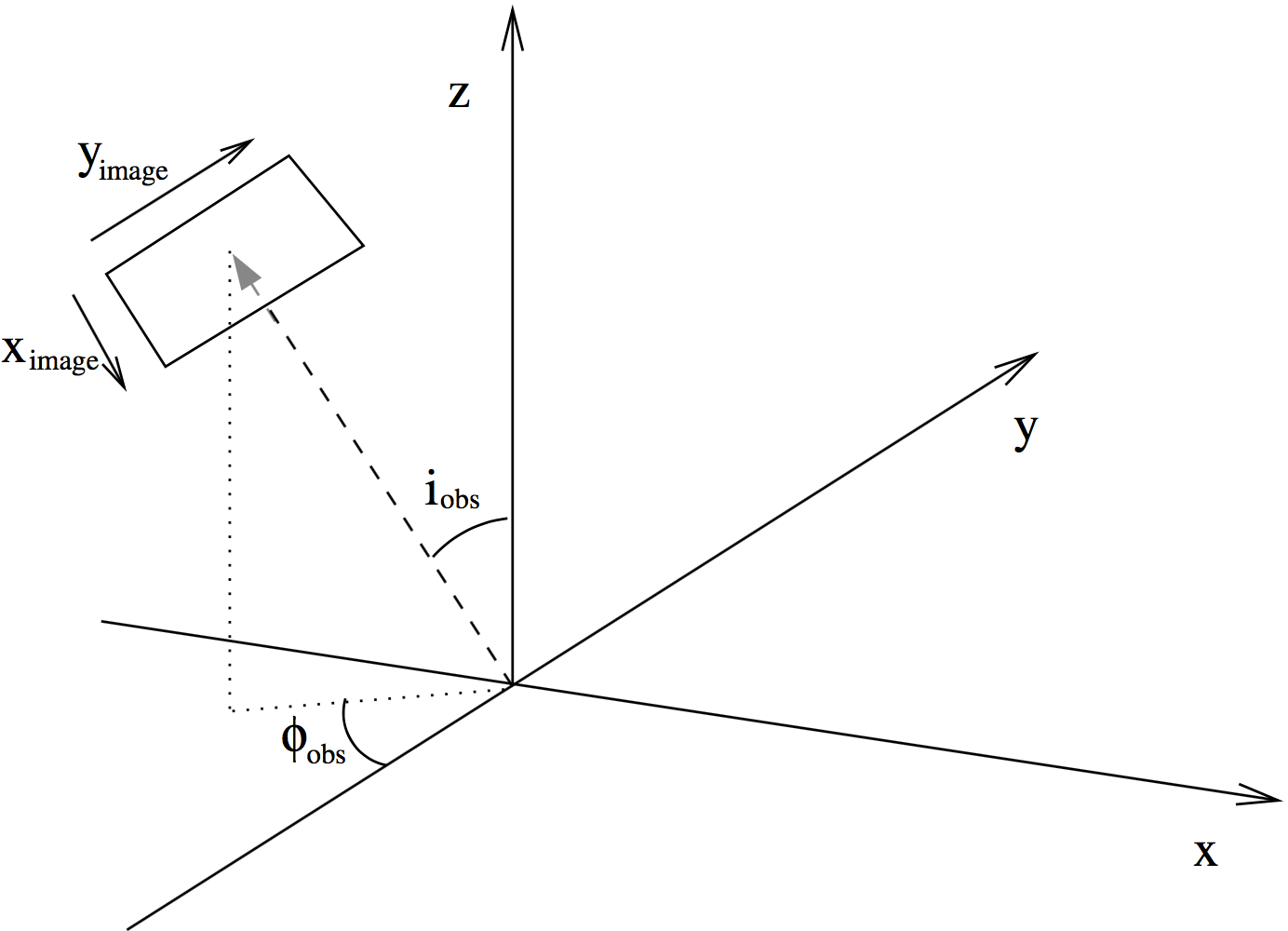
Fig. 9 Figure depicting how the angles ‘incl’ and ‘phi’ place the camera for images and spectra made with RADMC-3D. The code uses a right-handed coordinate system. The figure shows from which direction the observer is looking at the system, where \(i_{\mathrm{obs}}\) is the ‘incl’ keyword and \(\phi_{\mathrm{obs}}\) is the ‘phi’ keyword. The \(x_{\mathrm{image}}\) and \(y_{\mathrm{image}}\) are the horizontal (left-to-right) and vertical (bottom-to-top) coordinates of the image. For \(i_{\mathrm{obs}}=0\) and \(\phi_{\mathrm{obs}}=0\) the \(x_{\mathrm{image}}\) aligns with the 3-D \(x\)-coordinate and \(y_{\mathrm{image}}\) aligns with the 3-D \(y\)-coordinate.

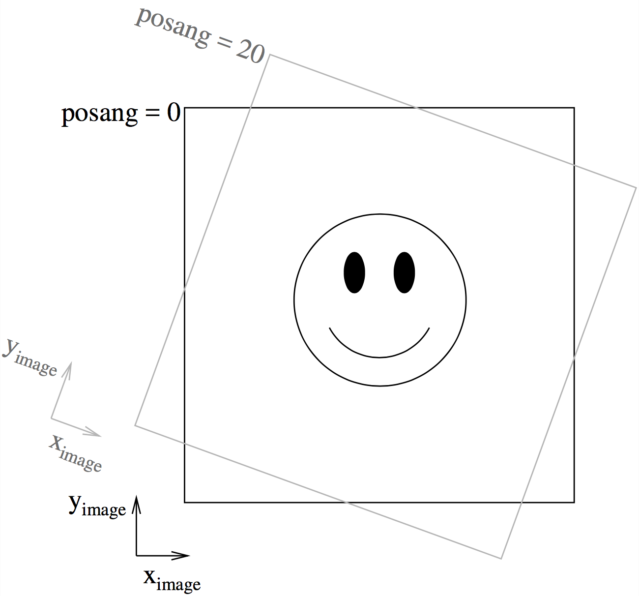
Fig. 10 This figure shows the way the camera can be rotated in the image plane using ‘posang’. Positive ‘posang’ means that the camera is rotated clockwise, so the object shown is rotated counter-clockwise with respect to the image coordinates.

You can also rotate the camera in the image plane with

radmc3d image lambda 10 incl 45 phi 30 posang 20

which rotates the camera by 20 degrees clockwise (i.e. the image rotates counter-clockwise). Figures Fig. 9 and Fig. 10 show the definitions of all three angles. Up to now the camera always pointed to one single point in space: the point (0,0,0). You can change this:

radmc3d image lambda 10 incl 45 phi 30 posang 20 pointau 3.2 0.1 0.4

which now points the camera at the point (3.2,0.1,0.4), where the numbers are in units of AU. The same can be done in units of parsec:

radmc3d image lambda 10 incl 45 phi 30 posang 20 pointpc 3.2 0.1 0.4

Note that pointau and pointpc are always 3-D positions specified in cartesian coordinates. This remains also true when the model-grid is in spherical coordinates and/or when the model is 2-D (axisymmetric) or 1-D (spherically symmetric): 3-D positions are always specified in x,y,z.

Let’s now drop the pointing again, and also forget about the posang, and try to change the number of pixels used:

radmc3d image lambda 10 incl 45 phi 30 npix 100

This will make an image of 100x100. You can also specify the x- and y- direction number of pixels separately:

radmc3d image lambda 10 incl 45 phi 30 npixx 100 npixy 30

Now let’s forget again about the number of pixels and change the size of the image, i.e. which zooming factor we have:

radmc3d image lambda 10 incl 45 phi 30 sizeau 30

This makes an image which has 30 AU width and 30 AU height (i.e. 15 AU from the center in both directions). Same can be done in units of parsec

radmc3d image lambda 10 incl 45 phi 30 sizepc 30

Although strictly speaking redundant is the possibility to zoom-in right into a selected box in this image:

radmc3d image lambda 10 incl 45 phi 30 zoomau -10 -4. 0 6

which means that we zoom in to the box given by \(-10\le x\le-4\) AU and \(0\le y\le 6\) AU on the original image (note that zoomau -15 15 -15 15 gives the identical result as sizeau 30). This possibility is strictly speaking redundant, because you could also change the pointau and sizeau to achieve the same effect (unless you want to make a non-square image, in which case this is the only way). But it is just more convenient to do any zooming-in this way. Please note that when you make non-square images with zoomau or zoompc, the code will automatically try to keep the pixels square in shape by adapting the number of pixels in x- or y- direction in the image and adjusting one of the sizes a tiny bit to assure that both x- and y- size are an integer times the pixel size. These are very small adjustments (and only take place for non-square zoom-ins). If you want to force the code to take exactly the zoom area, and you don’t care that the pixels then become slightly non-square, you can force it with truezoom:

radmc3d image lambda 10 incl 45 phi 30 sizeau 30 zoomau -10 -4. 0 3.1415 truezoom

If you do not want the code to adjust the number of pixels in x- and y- direction in its attempt to keep the pixels square:

radmc3d image lambda 10 incl 45 phi 30 sizeau 30 zoomau -10 -4. 0 3.1415 npixx 100 npixy 4 truepix

Now here are some special things. Sometimes you would like to see an image of just the dust, not including stars (for stars in the image: see Section Stars in the images and spectra). So blend out the stars in the image, you use the nostar option:

radmc3d image lambda 10 incl 45 phi 30 nostar

Another special option is to get a ‘quick image’, in which the code does not attempt assure flux conservation in the image (see Section The issue of flux conservation: recursive sub-pixeling for the issue of flux conservation). Doing the image with flux conservation is slower than if you make it without flux conservation. Making an image without flux conservation can be useful if you want to have a ‘quick look’, but is strongly discouraged for actual scientific use. But for a quick look you can do:

radmc3d image lambda 10 incl 45 phi 30 nofluxcons

If you want to produce images with a smoother look (and which also are more accurate), you can ask RADMC-3D to use second order integration for the images:

radmc3d image lambda 10 incl 45 phi 30 secondorder

NOTE: The resulting intensities may be slightly different from the case when first order integration (default) is used, in particular if the grid is somewhat course and the objects of interest are optically thick. Please consult Section Second order ray-tracing (Important information!) for more information.

Important for polarized radiative transfer: If you use polarized scattering, then you may want to creat images with polarization information in them. You have to tell RADMC-3D to do this by adding stokes to the command line:

radmc3d image lambda 10 incl 45 phi 30 stokes

The definitions of the Stokes parameters (orientation etc) can be found in Section Definitions and conventions for Stokes vectors and the format of image.out in this case can be found in Section OUTPUT: image.out or image_****.out.

Note: All the above commands call radmc3d separately. If it needs to load a large model (i.e. a model with many cells), then the loading may take a long time. If you want to make many images in a row, this may take too much time. Then it is better to call radmc3d as a child process and pass the above commands through the biway pipe (see Chapter chap-child-mode).

Making multi-wavelength images

Sometimes you want to have an image of an object at multiple wavelength simultaneously. Rather than calling RADMC-3D separately to make an image for each wavelength, you can make all images in one command. The only thing you have to do is to tell RADMC-3D which wavelengths it should take. There are various different ways you can tell RADMC-3D what wavelengths to take. This is described in detail in Section Specifying custom-made sets of wavelength points for the camera. Here we will focus as an example on just one of these methods. Type, for instance,

radmc3d image incl 45 phi 30 lambdarange 5. 20. nlam 10

This will create 10 images at once, all with the same viewing perspective, but at 10 wavelengths regularly distributed between 5 \(\mu`m and 20 :math:\)mu`m. All images are written into a single file, image.out (See Section OUTPUT: image.out or image_****.out for its format).

In Python you simply type:

from radmc3dPy import image
a=image.readImage()

and you will get all images at once. To plot one of them:

image.plotImage(image=a,ifreq=3)

which will plot image number 3 (out of images number 0 to 9). To find out which wavelength this image is at:

print(a.wav[3])

which will return 7.9370053 in this example.

Note that all of the commands in Section Basics of image making with RADMC-3D are of course also applicable to multi-wavelength images, except for the lambda keyword, as this conflicts with the other method(s) of specifying the wavlengths of the images. Now please turn to Section Specifying custom-made sets of wavelength points for the camera for more information on how to specify the wavelengths for the multiple wavelength images.

Making spectra

The standard way of making a spectrum with radmc3d is in fact identical to making 100x100 pixel images with flux conservation (i.e. recursive sub-pixeling, see Section The issue of flux conservation: recursive sub-pixeling) at multiple frequencies. You can ask radmc3d to make a spectral energy distribution (SED) with the command

radmc3d sed incl 45 phi 30

This will put the observer at inclination 45 degrees and angle phi 30 degrees, and make a spectrum with wavelength points equal to those listed in the wavelength_micron.inp file.

The output will be a file called spectrum.out (see Section OUTPUT: spectrum.out).

You can also make a spectrum on a set of wavelength points of your own choice. There are multiple ways by which you can specify the set of frequencies/wavelength points for which to make the spectrum: they are described in Section Specifying custom-made sets of wavelength points for the camera. If you have made your selection in such a way, you can make the spectrum at this wavelength grid by

radmc3d spectrum incl 45 phi 30 <COMMANDS FOR WAVELENGTH SELECTION>

where the last stuff is telling radmc3d how to select the wavelengths (Section Specifying custom-made sets of wavelength points for the camera). An example:

radmc3d spectrum incl 45 phi 30 lambdarange 5. 20. nlam 100

will make a spectrum with a regular wavelength grid between 5 and 20 \(\mu\mathrm{m}\) and 100 wavelength points. But see Section Specifying custom-made sets of wavelength points for the camera for more details and options.

The output file spectrum.out will have the same format as for the sed command.

Making a spectrum can take RADMC-3D some time, especially in the default mode, because it will do its best to shoot its rays to pick up all cells of the model (see Section The solution: recursive sub-pixeling). In particularly in spherical coordinates RADMC-3D can be perhaps too conservative (and thus slow). For spherical coordinates there are ways to tell RADMC-3D to be somewhat less careful (and thereby faster): see Section Recursive sub-pixeling in spherical coordinates.

Note that you can adjust the fine-ness of the images from which the spectrum is calculated using npix:

radmc3d sed incl 45 phi 30 npix 2

What this does is use a 2x2 pixel image instead of a 100x100 pixel image as the starting resolution. Of course, if it would really be just a 2x2 pixel image, the flux would be entirely unreliable and useless. However, using the above mentioned ‘sub-pixeling’ (see Section The solution: recursive sub-pixeling) it will automatically try to recursively refine these pixels until the required level of refinement is reached. So under normal circumstances even npix=2 is enough, and in earlier versions of RADMC-3D this 2x2 top-level image resolution was in fact used as a starting point. But for safety reasons this has now been changed to the standard 100x100 resolution which is also the default for normal images. If 100x100 is not enough, try e.g.:

radmc3d sed incl 45 phi 30 npix 400

which may require some patience.

What is ‘in the beam’ when the spectrum is made?

As mentioned above, a spectrum is simply made by making a rectangular image at all the wavelengths points, and integrating over these images. The resulting fluxes at each wavelength point is then the spectral flux at that wavelength point. This means that the integration area of flux for the spectrum is (a) rectangular and (b) of the same size at all wavelengths.

So, what is the size of the image that is integrated over? The answer is: it is the same size as the default size of an image. In fact, if you make a spectrum with

radmc3d spectrum incl 45 phi 30 lambdarange 5. 20. nlam 10

then this is the same as if you would type

radmc3d image incl 45 phi 30 lambdarange 5. 20. nlam 10

and read in the file image.out in into Python (see Section Making multi-wavelength images) or your favorite other data language, and integrate the images to obtain fluxes. In other words: the command spectrum is effectively the same as the command image but then instead of writing out an image.out file, it will integrate over all images and write a spectrum.out file.

If you want to have a quick look at the area over which the spectrum is to be computed, but you don’t want to compute all the images, just type e.g.:

radmc3d image lambda 10 incl 45 phi 30

then you see an image of your source at \(\lambda=10\mu\)m, and the integration area is precisely this area - at all wavelengths. Like with the images, you can specify your viewing area, and thus your integration area. For instance, by typing

radmc3d image lambda 10 incl 45 phi 30 zoomau -2 -1 -0.5 0.5

makes an image of your source at \(\lambda=10\mu\)m at inclination 45 degrees, and orientation 30 degrees, and zooms in at an are from -2 AU to -1 AU in x-direction (in the image) and from -0.5 AU to 0.5 AU in y-direction (in the image). To make an SED within the same integration area:

radmc3d sed incl 45 phi 30 zoomau -2 -1 -0.5 0.5

In this case we have an SED with a ‘beam size’ of 1 AU diameter, but keep in mind that the ‘beam’ is square, not circular.

Can one specify more realistic ‘beams’?

Clearly, a wavelength-independent beam size is unrealistic, and also the square beam is unrealistic. So is there a way to do this better? In reality one should really know exactly how the object is observed and how the flux is measured. If you use an interferometer, for instance, maybe your flux is meant to be the flux in a single synthesized beam. For a spectrum obtained with a slit, the precise flux is dependent on the slit width: the wider the slit, the more signal you pick up, but it is a signal from a larger area.

So if you really want to be sure that you know exactly what you are doing, then the best method is to do this youself by hand. You make multi-wavelength images:

radmc3d image incl 45 phi 30 lambdarange 5. 20. nlam 10

and integrate over the images in the way you think best mimics the actual observing procedure. You can do so, for instance, in Python. See Section Making multi-wavelength images for more information about multi-wavelength images.

But to get some reasonable estimate of the effect of the wavelength-dependent size and circular geometry of a ‘beam’, RADMC-3D allows you to make spectra with a simplistic circular mask, the radius of which can be specified as a function of wavelength in the file aperture_info.inp (see Section INPUT: aperture_info.inp). This file should contain a table of mask radii at various wavelengths, and when making a spectrum with the command-line keyword useapert the mask radii will be found from this table by interpolation. In other words: the wavelength points of the aperture_info.inp file do not have to be the same as those used for the spectrum. But their range must be larger or equal than the range of the wavelengths used for the spectrum, because otherwise interpolation does not work. In the most extreme simplistic case the aperture_info.inp file contains merely two values: one for a very short wavelength (shorter than used in the spectrum) and one for a very long wavelength (longer than used in the spectrum). The interpolation is then done double-logarithmically, so that a powerlaw is used between sampling points. So if you use a telescope with a given diameter for the entire range of the spectrum, two sampling points would indeed suffice.

You can now make the spectrum with the aperture in the following way:

radmc3d sed useapert dpc 100

The keyword dpc 100 is the distance of the observer in units of parsec, here assumed to be 100. This distance is necessary because the aperture information is given in arcseconds, and the distance is used to convert this is image size.

Important note: Although you specify the distance of the observer here, the spectrum.out file that is produced is still normalized to a distance of 1 parsec.

Note also that in the above example you can add any other keywords as shown in the examples before, as long as you add the useapert keyword and specify dpc.

A final note: the default behavior of RADMC-3D is to use the square field approach described before. You can explicitly turn off the use of apertures (which may be useful in the child mode of RADMC-3D) with the keyword noapert, but normally this is not necessary as it is the default.

Specifying custom-made sets of wavelength points for the camera

If you want to make a spectrum at a special grid of wavelengths/frequencies, with the spectrum command (see Section Making spectra), you must tell radmc3d which wavelengths you want to use. Here is described how to do this in various ways.

Using lambdarange and (optionally) nlam

The simplest way to choose a set of wavelength for a spectrum is with the lambdarange and (optionally) nlam command line options. Here is how to do this:

radmc3d spectrum incl 45 phi 30 lambdarange 5. 20.

This will make a spectrum between 5 and 20 \(\mu`m. It will use by default 100 wavelength points logarithmically spaced between 5 and 20 :math:\)mu`m. You can change the number of wavelength points as well:

radmc3d spectrum incl 45 phi 30 lambdarange 5. 20. nlam 1000

This will do the same, but creates a spectrum of 1000 wavelength points.

You can use the lambdarange and nlam options also for multi-wavelength images:

radmc3d image incl 45 phi 30 lambdarange 5. 20. nlam 10

but it is wise to choose nlam small, because otherwise the output file, containing all the images, would become too large.

Using allwl

You can also tell RADMC-3D to simply make an image at all of the wavelengths in the wavelength_micron.inp file:

radmc3d image incl 45 phi 30 allwl

The keyword allwl stands for ‘all wavelengths’.

Using loadcolor

By giving the command loadcolor on the command line, radmc3d will search for the file color_inus.inp. This file contains integers selecting the wavelengths from the file wavelength_micron.inp. The file is described in Section The color_inus.inp file (required with comm-line option ‘loadcolor’).

Using loadlambda

By giving the command loadlambda on the command line, radmc3d will search for the file camera_wavelength_micron.inp. This file contains a list of wavelengths in micron which constitute the grid in wavelength. This file is described in Section INPUT (optional): camera_wavelength_micron.inp.

Using iline, imolspec etc (for when lines are included)

By adding for instance iline 3 to the command line you specify a window around line number 3 (by default of molecule 1). By also specifying for instance imolspec 2 you select line 3 of molecule 2. By adding widthkms 3 you specify how wide the window around the line should be (3 km/s in this example). With vkms 2 you set the window offset from line center by 2 km/s in this example. By adding linenlam 30 you set the number of wavelength points for this spectrum to be 30 in this example. So a complete (though different) example is:

radmc3d spectrum incl 45 phi 30 iline 2 imolspec 1 widthkms 6.0 vkms 0.0 linenlam 40

Heads-up: In reality wavelength are actually wavelength bands

In a radiative transfer program like RADMC-3D the images or spectral fluxes are calculated at exact wavelengths. This would correspond to making observations with infinitely narrow filters, i.e. filters with \(\Delta\lambda=0\). This is not how real observations work. In reality each wavelength channel has a finite width \(\Delta\lambda\) and the measured flux (or image intensity) is an average over this range. To be even more precise, each wavelength channel \(i\) has some profile \(\Phi_i(\lambda)\) defined such that

\[\int_0^{\infty}\Phi_i(\lambda)d\lambda=1\]

For wide filters such as the standard photometric systems (e.g. UVBRI in the optical and JHK in the near infrared) these profiles span ranges with a width of the order of \(\lambda\) itself. Many instruments have their own set of filters. Usually one can download these profiles as digital tables. It can, under some circumstances, be important to include a treatment of these profiles in the model predictions. As an example take the N band. This is a band that includes the 10 \(\mu`m silicate feature, which is a strong function of wavelength *within* the N band. If you have a wide filter in the N band, then one cannot simply calculate the model spectrum in one single wavelength. Instead one has to calculate it for a properly finely sampled set of wavelengths :math:\)lambda_i` for \(1\le i\le n\), where \(n\) is the number of wavelength samples, and then compute the filter-averaged flux with:

\[F_{band} = \int_0^{\infty}\Phi_i(\lambda)F(\lambda)d\lambda = \sum_{i=1}^{n} \Phi_i F_i \delta\lambda\]

where \(\delta\lambda\) is the wavelength sampling spacing used. The same is true for image intensities. RADMC-3D will not do this automatically. You have to tell it the \(\lambda_i\) sampling points, let it make the images or fluxes, and you will then have to perform this sum yourself. Note that this will not always be necessary! In many (most?) cases the dust continuum is not expected to change so dramatically over the width of the filter that such degree of accuracy is required. So you are advised to think carefully: ‘do I need to take care of this or can I make do with a single wavelength sample for each filter?’. If the former, then do the hard work. If the latter: then you can save time.

Using channel-integrated intensities to improve line channel map quality

When you make line channel maps you may face a problem that is somehow related to the above issue of single-\(\lambda\)-sampling versus filter-integrated fluxes/intensities. If the model contains gas motion, then doppler shift will shift the line profile around. In your channel map you may see regions devoid of emission because the lines have doppler shifted out of the channel you are looking at. However, as described in Section What can go wrong with line transfer?, if the intrinsic line width of the gas is smaller than the cell-to-cell velocity differences, then the channel images may look very distorted (they will look ‘blocky’, as if there is a bug in the code). Please refer to Section What can go wrong with line transfer? for more details and updates on this important, but difficult issue. It is not a bug, but a general problem with ray-tracing of gas lines in models with large velocity gradients.

As one of the \(\beta\)-testers of RADMC-3D, Rahul Shetty, has found out, this problem can often be alleviated a lot if you treat the finite width of a channel. By taking multiple \(\lambda_i\) points in each wavelength channel (i.e. multiple \(v_i\) points in each velocity channel) and simply averaging the intensities (i.e. assuming a perfectly square \(\Phi\) function) and taking the width of the channels to be not smaller (preferably substantially wider) than the cell-to-cell velocity differences, this ‘blocky noise’ sometimes smoothes out well. However, it is always safer to use the ‘doppler catching’ mode (see Section Preventing doppler jumps: The ‘doppler catching method’) to automatically prevent such problems (though this mode requires more computer memory).

The issue of flux conservation: recursive sub-pixeling

The problem of flux conservation in images

If an image of nx\(\times\)ny pixels is made simply by ray-tracing one single ray for each pixel, then there is the grave danger that certain regions with high refinement (for instance with AMR in cartesian coordinates, or near the center of the coordinate system for spherical coordinates) are not properly ‘picked up’. An example: suppose we start with a circumstellar disk ranging from 0.1 AU out to 1000 AU. Most of the near infrared flux comes from the very inner regions near 0.1 AU. If an image of the disk is made with 100x100 pixels and image half-size of 1000 AU, then none of the pixels in fact pass through these very bright inner regions, for lack of spatial resolution. The problem is then that the image, when integrated over the entire image, does not have the correct flux. What should be is that the centermost pixels contain the flux from this innermost region, even if these pixels are much larger than the entire bright region. In other words, the intensity of these pixels must represent the average intensity, averaged over the entire pixel. Strictly speaking one should trace an infinite continuous 2-D series of rays covering the entire pixel and then average over all these rays; but this is of course not possible. In practice we should find a way to estimate the average intensity with only a finite number of rays.

The solution: recursive sub-pixeling

In RADMC-3D what we do is to use some kind of ‘adaptive grid refinement’ of the pixels of the image. For each pixel in the image the intensity is computed through a call to a subroutine called camera_compute_one_pixel(). In this subroutine a ray-tracing is performed for a ray that ends right in the middle of our pixel. During the ray-tracing, however, we check if we pass regions in the model grid that have grid cells with sizes \(S\) that are smaller than the pixel size divided by some factor \(f_{\mathrm{ref}}\) (where pixel size is, like the model grid size S itself, measured in centimeters. If this is found not to be true, then the pixel size was apparently ok, and the intensity resulting from the ray-tracing is now returned as the final intensity of this pixel. If, however, this condition is found to be true, then the result of this ray is rejected, and instead 2x2 sub-pixels are computed by calling the camera_compute_one_pixel() subroutine recursively. We thus receive the intensity of each of these four sub-pixels, and we return the average of these 4 intensities.

Note, by the way, that each of these 2x2 subpixels may be split even further into 2x2 sub-pixels etc until the desired resolution is reached, i.e. until the condition that \(S\) is larger or equal to the pixel size divided by \(f_{\mathrm{ref}}\) is met. This is illustrated in Fig. Fig. 11. By this recursive calling, we always end up at the top level with the average intesity of the entire top-level pixel. This method is very similar to quad-tree mesh refinement, but instead of retaining and returning the entire complex mesh structure to the user, this method only returns the final average intensity of each (by definition top level) pixel in the image. So the recursive sub-pixeling technique described here is all done internally in the RADMC-3D code, and the user will not really notice anything except that this sub-pixeling can of course be computationally more expensive than if such a method is not used.

Fig. 11 Pictographic representation of how the recursive sub-pixeling for images works. Pixels are recursively split in 2x2 subpixels as far as needed to resolve the 3-D grid structure of the model. But at the end, the fluxes of all subpixels are summed up such that the resulting image has a regular grid again.

Note that the smaller we choose \(f_{\mathrm{ref}}\) the more accurate our image becomes. In the radmc3d.inp file the value of \(f_{\mathrm{ref}}\) can be set by setting the variable camera_refine_criterion to the value you want \(f_{\mathrm{ref}}\) to be. Not setting this variable means RADMC-3D will use the default value which is reasonable as a choice (default is 1.0). The smaller you set camera_refine_criterion, the more accurate and reliable the results become (but the heavier the calculation becomes, too).

NOTE: The issue of recursive sub-pixeling becomes tricky when stars are treated as spheres, i.e. non-point-like (see Section Stars in the images and spectra and Chapter More information about the treatment of stars).

NOTE: If you want to know, for a given image, how RADMC-3D subpixeled the image, you can either set camera_diagnostics_subpix=1 in the radmc3d.inp file or add diag_subpix to the command line. This forces RADMC-3D to write out a file called subpixeling_diagnostics.out which contains four columns, for respectivly: px,py,pdx,pdy, i.e. the pixel position and its size. This allows the user to find out if the recursive subpixeling went well or if certain areas were over/under-resolved. This is really only meant as a diagnostic.

A danger with recursive sub-pixeling

It is useful to keep in mind that for each pixel the recursive sub-pixeling is triggered if the ray belonging to that pixel encounters a cell that is smaller than the pixel size. This normally works well if \(f_{\mathrm{ref}}\) is chosen small enough. But if there exist regions in the model where one big non-refined cell lies adjacent to a cell that is refined, say, 4 times (meaning the big cell has neighbors that are 16 times smaller!), then if the ray of the pixel just happens to miss the small cells and only passes the big cell, it won’t ‘notice’ that it may need to refine to correctly capture the tiny neighboring cells accurarely.

Such a problem only happens if refinement levels jump by more than 1 between adjacent cells. If so, then it may be important to make \(f_{\mathrm{ref}}\) correspondingly smaller (by setting camera_refine_criterion in radmc3d.inp to the desired value). A bit of experimentation may be needed here.

Recursive sub-pixeling in spherical coordinates

In spherical coordinates the recursive sub-pixeling has a few issues that you may want to be aware of. First of all, in 1-D spherical coordinates each cell is in fact a shell of a certain thickness. In 2-D spherical coordinates cells are rings. In both cases the cells are not just local boxes, but have 2 or 1 (respectively) extended dimensions. RADMC-3D takes care to still calculate properly how to define the recursive sub-pixeling scale. But for rays that go through the central cavity of the coordinate system there is no uniquely defined pixel resolution to take. The global variable camera_spher_cavity_relres (with default value 0.05) defines such a relative scale. You can change this value in the radmc3d.inp file.

A second issue is when the user introduces extreme ‘separable refinement’ (see Section Separable grid refinement in spherical coordinates (important!) and Figure Fig. 23) in the \(R\), \(\Theta\) or \(\Phi\) coordinate. This may, for instance, be necessary near the inner edge of a dusty disk model in order to keep the first cell optically thin. This may lead, however, to extremely deep sub-pixeling for rays that skim the inner edge of the grid. This leads to a huge slow-down of the ray-tracing process although it is likely not to give much a different result. By default RADMC-3D plays it safe. If you wish to prevent this excessive sub-pixeling (at your own risk) then you can set the following variables in the radmc3d.inp file:

• camera_min_drr which sets a lower limit to the \(\Delta R/R\) taken into account for the sub-pixeling (region ‘B’ in Figure Fig. 22). The default is 0.003. By setting this to e.g. 0.03 you can already get a strong speed-up for models with strong \(R\)-refinement.

• camera_min_dangle which sets a lower limit to \(\Delta\Theta\) (region ‘C’ in Figure Fig. 22) and/or \(\Delta\Phi\). The default is 0.05. By setting this to e.g. 0.1 you can already get some speed-up for models with e.g. strong \(\Theta\)-refinement.

It is important to keep in mind that the smaller you make this number, the more accurate and reliable the results. It may be prudent to experiment with smaller values of camera_min_drr for models with extremely optically thick inner edges, e.g. a protoplanetary disk with an abrupt inner edge and a high dust surface density. For a disk model with a very thin vertical extent it will be important to choose small values of camera_min_dangle, perhaps even smaller than the default value.

For your convenience: Because it can be sometimes annoying to always have to play with the camera_min_drr, camera_min_dangle and camera_spher_cavity_relres values, and since it is usually (!) not really necessary to have such extremely careful subpixeling, RADMC-3D now has a new command line option called sloppy. This command-line option will set: camera_min_drr=0.1, camera_min_dangle=0.1 and camera_spher_cavity_relres=0.1. So if you have an image like this:

radmc3d image lambda 10 incl 45 phi 30 sloppy

then it will make the image with moderate, but not excessive subpixeling. This may, under some circumstances, speed up the image-making in spherical coordinates by a large factor. Similar for making spectra. For instance:

radmc3d sed incl 45 phi 30 sloppy

can be, under some circumstances, very much faster than without the sloppy option.

Note,however, that using the sloppy option and/or setting the values of camera_min_drr, camera_min_dangle and camera_spher_cavity_relres in the radmc3d.inp file by hand, {bf is all at your own risk!} It is always prudent to check your results, now and then, against a non-sloppy calculation.

How can I find out which pixels RADMC-3D is recursively refining?

Sometimes you notice that the rendering of an image or spectrum takes much more time than you expected. When recursive sub-pixeling is used for imaging, RADMC-3D will give diagnostic information about how many more pixels it has rendered than the original image resolution. This factor can give some insight if extreme amount of sub-pixeling refinement has been used. But it does not say where in the image this occurs. If you want to see exactly which pixels and subpixels RADMC-3D has rendered for some image, you can use the following command-line option:

radmc3d image lambda 10 diag_subpix

This diag_subpix option will tell RADMC-3D to write a file called subpixeling_diagnostics.out which contains four columns: One for the x-coordinate of the (sub-)pixel, one for the y-coordinate of the (sub-)pixel, one for the x-width of the (sub-)pixel and a final one for the y-width of the (sub-)pixel. In Python you can then use, for instance, the Numpy loadtxt method to read these columns.

If this diagnostic shows that the subpixeling is excessive (which can particularly happen in spherical coordinates) then you might want to read Section Recursive sub-pixeling in spherical coordinates.

Alternative to recursive sub-pixeling

As an alternative to using this recursive sub-pixeling technique to ensure flux conservation for images, one can simply enhance the spatial resolution of the image, for instance

radmc3d image lambda 10 npix 400

Or even 800 or so. This has the clear advantage that the user gets the complete information of the details in the image (while in the recursive sub-pixeling technique only the averages are retained). The clear disadvantages are that one may need rediculously high-resolution images (i.e. large data sets) to resolve all the details and one may waste a lot of time rendering parts of the image which do not need that resolution. The latter is typically an issue when images are rendered from models that use AMR techniques.

Stars in the images and spectra

Per default, stars are still treated as point sources. That means that none of the rays of an image can be intercepted by a star. Starlight is included in each image as a post-processing step. First the image is rendered without the stars (though with of course all the emission of dust, lines etc induced by the stars) and then for each star a ray tracing is done from the star to the observer (where only extinction is taken into account, because the emission is already taken care of) and the flux is then added to the image at the correct position. You can switch off the inclusion of the stars in the images or spectra with the nostar command line option.

However, as of version 0.17, stars can also be treated as the finite-size spheres they are. This is done with setting istar_sphere = 1 in radmc3d.inp. However, this mode can slow down the code a bit or even substantially. And it may still be partly under development, so the code may stop if it is required to handle a situation it cannot handle yet. See Chapter More information about the treatment of stars for details.

Second order ray-tracing (Important information!)

Ideally we would like to assure that the model grid is sufficiently finely spaced everywhere. But in many cases of interest one does not have this luxury. One must live with the fact that, for memory and/or computing time reasons, the grid is perhaps a bit coarser than would be ideal. In such a case it becomes important to consider the ‘order’ of integration of the transfer equation. By default, for images and spectra, RADMC-3D uses first order integration: The source term and the opacity in each cell are assumed to be constant over the cell. This is illustrated in Fig. Fig. 12.

Fig. 12 Pictographic representation of the first order integration of the transfer equation along a ray (red line with arrow head) through an AMR grid (black lines). The grid cuts the ray into ray segments A, B, C and D. At the bottom it is shown how the integrands are assumed to be along these four segments. The emissivity function \(j_\nu\) and extinction function \(\alpha_\nu\) are constant within each cell and thus constant along each ray segment.

The integration over each cell proceeds according to the following formula:

\[I_{\mathrm{result}} = I_{\mathrm{start}}e^{-\tau} + (1-e^{-\tau})S\]

where \(S=j/\alpha\) is the source function, assumed constant throughout the cell, \(\tau=\alpha\,\Delta s\) is the optical depth along the path that the ray makes through the cell, and \(I_{\mathrm{start}}\) is the intensity upon entering the cell. This is the default used by RADMC-3D because the Monte Carlo methods also treat cells as having constant properties over each cell. This type of simple integration is therefore the closest to how the Monte Carlo methods (thermal MC, scattering MC and mono MC) ‘see’ the grid. However, with first order integration the images look somewhat ‘blocky’: you can literally see the block structure of the grid cells in the image, especially if you make images at angles aligned with the grid. For objects with high optical depths you may even see grid patterns in the images.

RADMC-3D can also use second order integration for its images and spectra. This is illustrated in Fig. Fig. 13.

Fig. 13 Pictographic representation of the second order integration of the transfer equation along a ray (red line with arrow head) through an AMR grid (black lines). The grid cuts the ray into ray segments A, B, C and D. At the bottom it is shown how the integrands are assumed to be along these four segments. The emissivity function \(j_\nu\) and extinction function \(\alpha_\nu\) are given at the cell corners (solid blue circles), and linearly interpolated from the cell corners to the locations where the ray crosses the cell walls (open blue circles). Then, along each ray segment the emissivity and extinction functions are assumed to be linear functions, so that the integration result is quadratic.

This is done with a simple secondorder option added on the command line, for instance:

radmc3d image lambda 10 secondorder

The integration now follows the formula (Olson et al. 1986):

\[I_{\mathrm{result}} = I_{\mathrm{start}}e^{-\tau} + (1-e^{-\tau}-\beta) S_{\mathrm{start}} + \beta S_{\mathrm{end}}\]

with

\[\beta = \frac{\tau-1+e^{-\tau}}{\tau}\]

and

\[\tau = \frac{\alpha_{\mathrm{start}}+\alpha_{\mathrm{end}}}{2}\Delta s\]

For \(\tau\rightarrow 0\) we have the limit \(\beta\rightarrow \tau/2\), while for \(\tau\rightarrow \infty\) we have the limit \(\beta\rightarrow 1\).

The values of \(\alpha\), \(S\) etc., at the ‘start’ position are obtained at the cell interface where the ray enters the cell. The values at the ‘end’ position are obtained at the cell interface where the ray leaves the cell. The above formulas represent the exact solution of the transfer equation along this ray-section if we assume that all variables are linear functions between the ‘start’ and ‘end’ positions.

The next question is: How do we determine the physical variables at the cell interfaces (‘start’ and ‘end’)? After all, initially all variables are stored for each cell, not for each cell interface or cell corner. The way that RADMC-3D does this is:

• First create a ‘grid of cell corners’, which we call the vertex grid (see the solid blue dots in Fig. Fig. 13). The cell grid already implicitly defines the locations of all the cell corners, but these corners are, by default, not explicitly listed in computer memory. When the secondorder option is given, however, RADMC-3D will explicitly find all cell corners and assign an identity (a unique integer number) to each one of them. NOTE: Setting up this vertex grid costs computer memory!

• At each vertex (cell corner) the physical variables of the (up to) 8 cells touching the vertex are averaged with equal weight for each cell. This now maps the physical variables from the cells to the vertices.

• Whenever a ray passes through a cell wall, the physical variables of the 4 vertices of the cell wall are interpolated bilinearly onto the point where the ray passes through the cell wall (see the open blue circles in Fig. Fig. 13). This gives the values at the ‘start’ or ‘end’ points.

• Since the current ‘end’ point will be the ‘start’ point for the next ray segment, the physical variables need only be obtained once per cell wall, as they can be recycled for the next ray segment. Each set of physical variables will thus be used twice: once for the ‘end’ and once for the ‘start’ of a ray segment (except of course at the very beginning and very end of the ray).

Fig. 14 First-order integration of transfer equation in ray-tracing seen at inclination 4 degrees.

Fig. 15 First-order integration of transfer equation in ray-tracing seen at inclination 60 degrees.

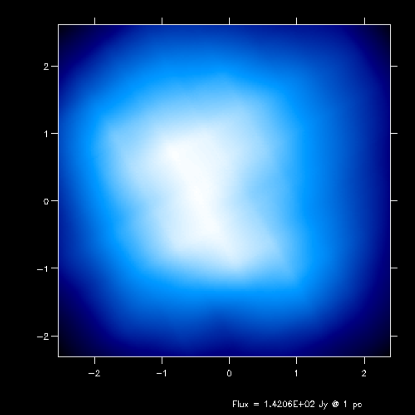
Fig. 16 Second-order integration of transfer equation in ray-tracing seen at inclination 4 degrees.

Fig. 17 Second-order integration of transfer equation in ray-tracing seen at inclination 60 degrees.

If you compare the images or spectra obtained with first order integration (default, see Figs. Fig. 16 and Fig. 17) or second order integration (see Figs. Fig. 16 and Fig. 17) you see that with the first order method you still see the cell structure of the grid very much. Also numerical noise in the temperature due to the Monte Carlo statistics is much more prominent in the first order method. The second order method makes much smoother results.

For line transfer the second order mode can be even improved with the ‘doppler catching method’, see Section Preventing doppler jumps: The ‘doppler catching method’.

WARNING: Second order integration for the images and spectra from dust continuum emission can in some cases lead to overestimation of the fluxes. This is because the dust temperature calculated using the thermal Monte Carlo algorithm assumes the temperature to be constant over each cell. The second order integration for the images and spectra will, however, smear the sources a bit out. This then leads to ‘leaking’ of emissivity from optically thick cells into optically thin cells. These optically thin cells can then become too bright.

Second order integration in spherical coordinates: a subtle issue

The second order integration (as well as the doppler-catching method, see Section Preventing doppler jumps: The ‘doppler catching method’) work in cartesian coordinates as well as in spherical coordinates. In spherical coordinates in 1-D (spherical symmetry) or 2-D (axial symmetry) there is, however, a very subtle issue that can lead to inaccuracies, in particular with line transfer. The problem arises in the cell where a ray reaches its closest approach to the origin of the coordinate system (or closest approach to the symmetry axis). There the ray segment can become fairly long, and its angle with respect to the symmetry axis and/or the origin can drastically change within this single ray-segment. This can sometimes lead to inaccuracies.

As of version 0.41 of RADMC-3D a new global variable is introduced, camera_maxdphi, which has as default the value 0.1, but which can be set to another value in the radmc3d.inp file. It sets the maximum angle (in radian) which a ray segment in spherical coordinates is allowed to span with respect to the origin of the coordinate system. If a ray segment spans an angle larger than that, the ray-segment is cut into smaller segments. This means that in that cell the ray will consist of more than one segment.

If camera_maxdphi=0 this segment cutting is switched off (for backward compatibility to earlier versions of RADMC-3d).

Circular images

RADMC-3D offers (optionally!) an alternative to the usual x-y rectangular pixel arrangement of images: circular images. Here the pixels are not arranged in rows that are vertically stacked \((x,y)\), but in concentric circles \((r,\phi)\). Such a pixel arrangement is, of course, radically different from what we usually consider “an image”, and it is therefore not possible to view such an image with the usual image viewing methods (such as Python’s plt.imshow()). Or more precisely: if you would use plt.imshow() on a circular image you would see something that you would not recognize as the image it should represent.

So what is the purpose? It is useful for models created on a spherical coordinate system. Such models can have structure at a huge range of scales, from very tiny (at the small-end side of the radius coordinate \(r\)) to very large (at the large-end side of the radius coordinate \(r\)). If you make a normal image, you have to pick the right “zoom factor”: are you interested to see the outer regions or more interested in the inner regions? If you choose a “zoomed out” image, you will under-resolve the inner regions. If you choose a “zoomed in” image, you will not see the outer regions (they are beyond the edge of the image). One solution could be to choose a huge number of pixels, but that would create huge image files.

Circular images solve this dilemma. By arranging the pixels not in \((x,y)\) but instead of \((r,\phi)\), the \(r\) coordinate grid of the image will automatically be adapted to the \(r\) coordinate grid of the spherical coordinate system. If the latter is logarithmically spaced, so will the circular image.

Here is how it works: Assuming you have a model in spherical coordinates, you can create a circular image as follows:

radmc3d image circ lambda 10

which creates a circular image at wavelength \(\lambda=10\mu m\).

Using radmc3dPy you can read this image as follows:

from radmc3dPy import image
im = image.readcircimage()

The data is now in im.image. A radial plot of the intensity at a given angle \(\phi\) could be made as follows:

import matplotlib.pyplot as plt
plt.loglog(im.rc,im.image[:,0,0,0])
plt.xlabel('r [cm]')
plt.ylabel(r'$I_\nu [erg\, cm^{-2}\, s^{-1}\, Hz^{-1}\, ster^{-1}]$')

The result will look like shown in Fig. Fig. 18 .

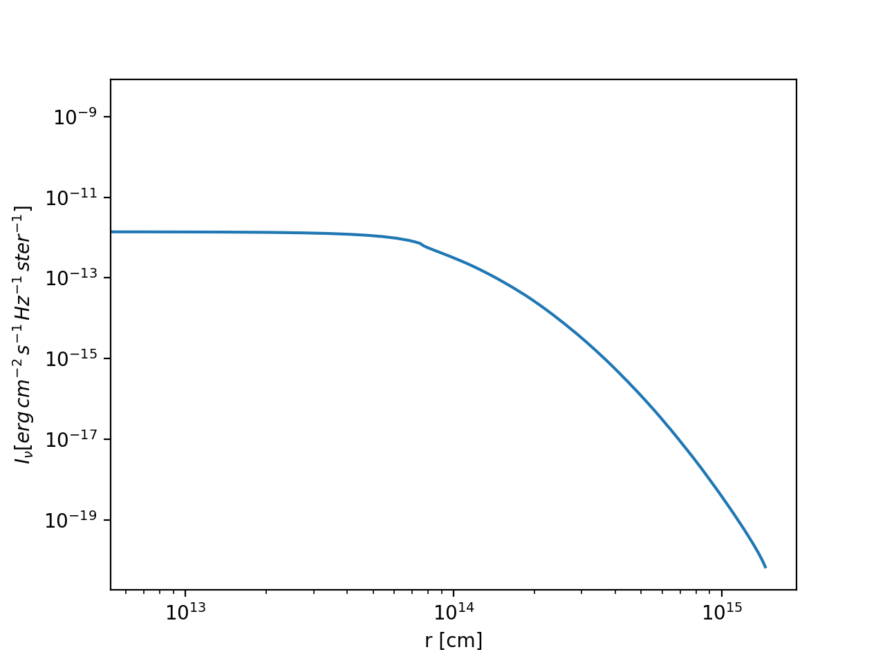
Fig. 18 Example of a circular image of a 1-D spherical model (the model in the examples/run_spher1d_1/ directory).

If you have 2-D or 3-D models in spherical coordinates, the circular images (should) have not only a grid in \(r\), but also \(\phi\) grid points. A simple plot such as Fig. Fig. 18 will only show the intensity for a single \(phi\) choice. There is no “right” or “wrong” way of displaying such an image. It depends on your taste. You could, of course, remap onto a “normal” image, but that would defeat the purpose of circular images. You could also display the \((r,\phi)\) image directly with e.g. plt.imshow(), which simply puts the \(r\) axis horizontally on the screen, and the \(\phi\) axis vertically, essentially creating a ‘heat map’ of the intensity as a function of \(r\) and \(\phi\).

This is illustrated in the model examples/run_spher2d_1/. Fig. Fig. 19 shows the circular image (as a ‘heat map’) at a wavelength of \(\lambda=10\;\mu m\). For comparison, the same image is shown as a ‘normal’ image in Fig. Fig. 20.

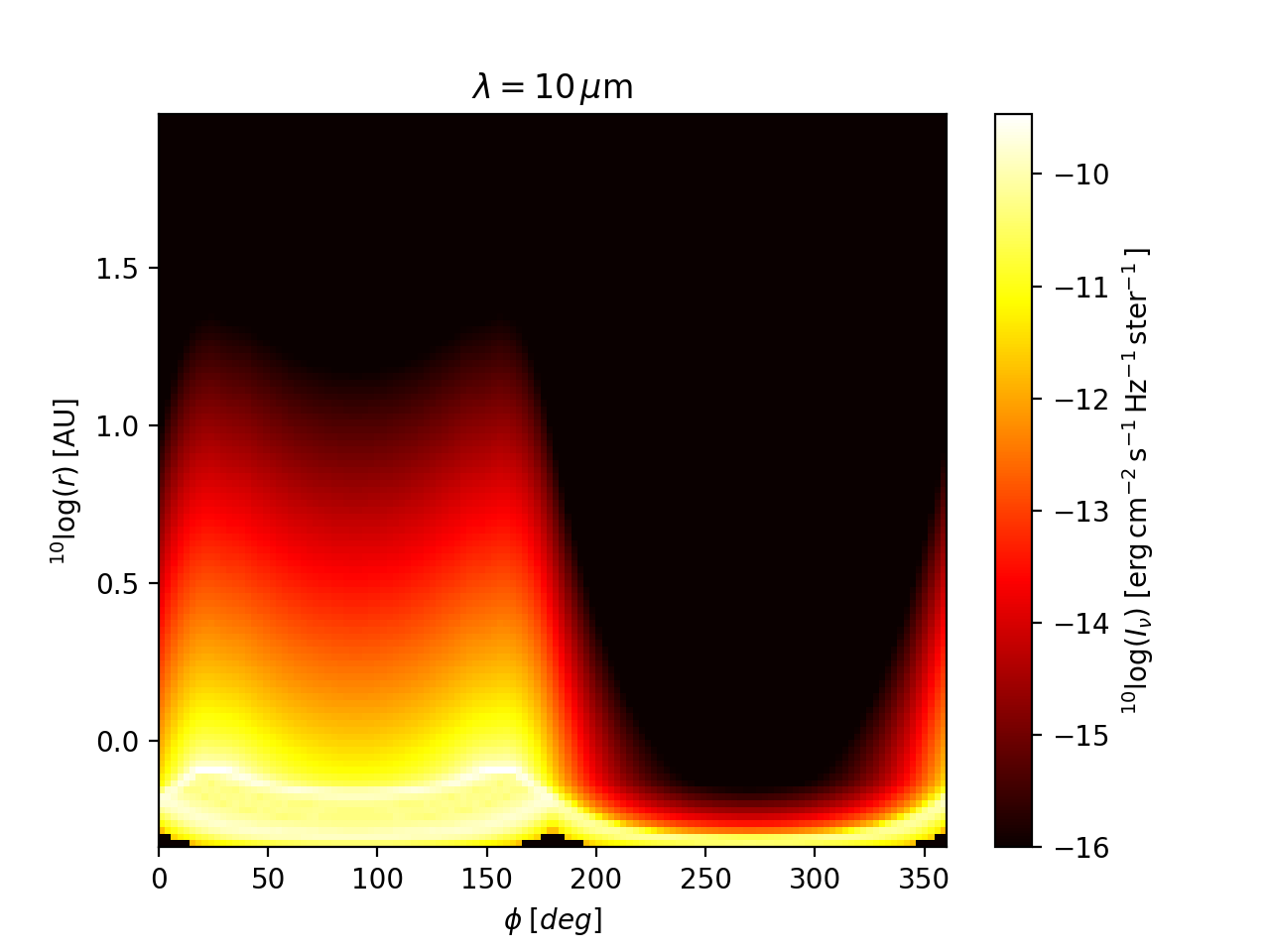
Fig. 19 Example of a circular image of a 2-D spherical model (the model in the examples/run_spher2d_1/ directory).

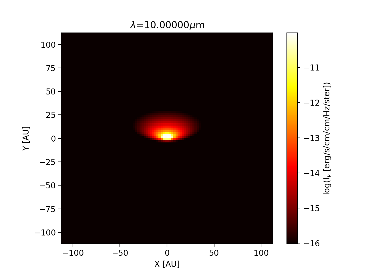
Fig. 20 The rectangular (‘normal’) version of the image of Fig. Fig. 19. As one can see: the inner regions of this image are not well-resolved.

With a bit of “getting used to” one will find that the circular images will reveal a lot of information.

Note: Fig. :numfig:`fig-circ-image-2d` shows an effect similar to what is shown in Fig. Fig. 30. This indicates that near the inner radius of the model, the radial grid is under-resolved in example model examples/run_spher2d_1/: see Section Careful: Things that might go wrong, point ‘Too optically thick cells at the surface or inner edge’. So, to improve the reliability of model examples/run_spher2d_1/, one would need to refine the radial grid near the inner edge and/or smooth the density there.

Visualizing the \(\tau=1\) surface

To be able to interpret the outcome of the radiative transfer calculations it is often useful to find the spatial location of the \(\tau=1\) surface (or, for that matter, the \(\tau=0.1\) surface or any \(\tau=\tau_s\) surface) as seen from the vantage point of the observer. This makes it easier to understand where the emission comes from that you are seeing. RADMC-3D makes this possible. Thanks to Peter Schilke and his team, for suggesting this useful option.

The idea is to simply replace the command-line keyword image with tausurf 1.0. The \(1.0\) stands for \(\tau_s=1.0\), meaning we will find the \(\tau=1.0\) surface. Example: Normally you might make an image with e.g. the following command:

radmc3d image lambda 10 incl 45 phi 30

Now you make a \(\tau=1\) surface with the command:

radmc3d tausurf 1.0 lambda 10 incl 45 phi 30

or a \(\tau=0.2\) surface with

radmc3d tausurf 0.2 lambda 10 incl 45 phi 30

The image output file image.out will now contain, for each pixel, the position along the ray in centimeters where \(\tau=\tau_s\). The zero point is the surface perpendicular to the direction of observation, going through the pointing position (which is, by default \((0,0,0)\), but see the description of pointau in Section Basics of image making with RADMC-3D). Positive values mean that the surface is closer to the observer than the plane, while negative values mean that the surface is behind the plane.

If, for some pixel, there exists no \(\tau=\tau_s\) point because the total optical depth of the object for the ray belonging to that pixel is less than \(\tau_s\), then the value will be -1e91.

You can also get the 3-D (i.e. \(x\), \(y\), \(z\)) positions of each of these points on the \(\tau=\tau_s\) surface. They are stored in the file tausurface_3d.out.

Note that if you make multi-frequency images, you will also get multi-frequency \(\tau=\tau_s\) surfaces. This can be particularly useful if you want to understand the sometimes complex origins of the shapes of molecular/atomic lines.

You can also use this option in the local observer mode, though I am not sure how useful it is. Note, however, that in that mode the value stored in the image.out file will describe the distance in centimeter to the local observer. The larger the value, the farther away from the observer (contrary to the case of observer-at-infinity).

Example usage:

radmc3d tausurf 1 lambda 10 incl 45 phi 30

Maps of optical depth \(\tau\)

Another way to get a better understanding of the optical depth of your model is to make an “image of optical depths”. It is just like making an image, but instead of each pixel containing the intensity \(I_\nu\) of the image, each pixel now contains the full optical depth \(\tau_\nu\) along the ray. In this way you get an optical depth map.

The idea is to simply make an image, as you would normally do, but now add the command-line keyword tracetau. Example:

radmc3d image lambda 10 incl 45 phi 30 tracetau

The image output file image.out will now contain, for each pixel, the optical depth.

You can also use the command-line keyword tracecolumn, in which case your image will not contain the optical depth, but the total column density. Note: For now it only includes the column density of the dust.

For public outreach work: local observers inside the model

While it may not be very useful for scientific purposes (though there may be exceptions), it is very nice for public outreach to be able to view a model from the inside, as if you, as the observer, were standing right in the middle of the model cloud or object. One can then use physical or semi-physical or even completely ad-hoc opacities to create the right ‘visual effects’. RADMC-3D has a viewing mode for this purpose. You can use different projections:

• Projection onto flat screen:

  The simplest one is a projection onto a screen in front (or behind) the point-location of the observer. This gives an image that is good for viewing in a normal screen. This is the default (camera_localobs_projection=1).

• Projection onto a sphere:

  Another projection is a projection onto a sphere, which allow fields of view that are equal or larger than \(2\pi\) of the sky. It may be useful for projection onto an OMNIMAX dome. This is projection mode camera_localobs_projection=2.

You can set the variable camera_localobs_projection to 1 or 2 by adding on the command line projection 2 (or 1), or by setting it in the radmc3d.inp as a line camera_localobs_projection = 2 (or 1).

To use the local projection mode you must specify the following variables on the command line:

• sizeradian: This sets the size of the image in radian (i.e. the entire width of the image). Setting this will make the image width and height the same (like setting sizeau in the observer-at-infinity mode, see Section Basics of image making with RADMC-3D).

• zoomradian: Instead of sizeradian you can also specify zoomradian, which is the local-observer version of zoomau or``zoompc`` (see Section Basics of image making with RADMC-3D).

• posang: The position angle of the camera. Has the same meaning as in the observer-at-infinity mode.

• locobsau or locobspc: Specify the 3-D location of the local observer inside the model in units of AU or parsec. This requires 3 numbers which are the x, y and z positions (also when using spherical coordinates for the model setup: these are still the cartesian coordinates).

• pointau or pointpc: These have the same meaning as in the observer-at-infinity model. They specify the 3-D location of the point of focus for the camera (to which point in space is the camera pointing) in units of AU or parsec. This requires 3 numbers which are the x, y and z positions (also when using spherical coordinates for the model setup: these are still the cartesian coordinates).

• zenith (optional): For Planetarium Dome projection (camera_localobs_projection=2) it is useful to make the pointing direction not at the zenith (because then the audience will always have to look straight up) but at, say, 45 degrees. You can facilitate this (optionally) by adding the command line option zenith 45 for a 45 degrees offset. This means that if you are sitting under the OMNIMAX dome, then the camera pointing (see pointau above) is 45 degrees in front of you rather than at the zenith. This option is highly recommended for dome projections, but you may need to play with the angle to see which gives the best effect.

Setting sizeradian, zoomradian, locobsau or locobspc on the command line automatically switches to the local observer mode (i.e. there is no need for an extra keyword setting the local observer mode on). To switch back to observer-at-infinity mode, you specify e.g. incl or phi (the direction toward which the observer is located in the observer-at-infinity mode). Note that if you accidently specify both e.g. sizeradian and incl, you might end up with the wrong mode, because the mode is set by the last relevant entry on the command line.

The images that are produced using the local observer mode will have the x- and y- pixel size specifications in radian instead of cm. The first line of an image (the format number of the file) contains then the value 2 (indicating local observer image with pixel sizes in radian) instead of 1 (which indicates observer-at-infinity image with pixel sizes in cm).

NOTE: For technical reasons dust scattering is (at least for now) not included in the local observer mode! It is discouraged to use the local observer mode for scientific purposes.

Multiple vantage points: the ‘Movie’ mode

It can be useful, both scientifically and for public outreach, to make movies of your model, for instance by showing your model from different vantage points or by ‘travelling’ through the model using the local observer mode (Section For public outreach work: local observers inside the model). For a movie one must make many frames, each frame being an image created by RADMC-3D’s image capabilities. If you call radmc3d separately for each image, then often the reading of all the large input files takes up most of the time. One way to solve this is to call radmc3d in ‘child mode’ (see Chapter chap-child-mode). But this is somewhat complicated and cumbersome. A better way is to use RADMC-3D’s ‘movie mode’. This allows you to ask RADMC-3D to make a sequence of images in a single call. The way to do this is to call radmc3d with the movie keyword:

radmc3d movie

This will make radmc3d to look for a file called movie.inp which contains the information about each image it should make. The structure of the movie.inp file is:

iformat
nframes
<<information for frame 1>>
<<information for frame 2>>
<<information for frame 3>>
...
<<information for frame nframes>>

The iformat is an integer that is described below. The nframes is the number of frames. The <<information for frame xx>> are lines containing the information of how the camera should be positioned for each frame of the movie (i.e. for each imag). It is also described below.

There are multiple ways to tell RADMC-3D how to make this sequence of images. Which if these ways RADMC-3D should use is specified by the iformat number. Currently there are 2, but later we may add further possibilities. Here are the current possibilities

• iformat=1: The observer is at infinity (as usual) and the <<information for frame xx>> consists of the following numbers (separated by spaces):

  pntx pnty pntz hsx hsy pa incl phi
  

  These 8 numbers have the following meaning:

  • pntx,pnty,pntz: These are the x, y and z coordinates (in units of cm) of the point toward which the camera is pointing.

  • hsx,hsy: These are the image half-size in horizontal and vertical direction on the image (in units of cm).

  • pa: This is the position angle of the camera in degrees. This has the same meaning as for a single image.

  • incl,phi: These are the inclination and phi angle toward the observer in degrees. These have the same meaning as for a single image.

• iformat=-1: The observer is local (see Section For public outreach work: local observers inside the model) and the <<information for frame xx>> consists of the following numbers (separated by spaces):

  pntx pnty pntz hsx hsy pa obsx obsy obsz
  

  These 9 numbers have the following meaning:

  • pntx,pnty,pntz,hsx,hsy,pa: Same meaning as for iformat=1.

  • obsx,obsy,obsz: These are the x, y and z position of the local observer (in units of cm).

Apart from the quantities that are thus set for each image separately, all other command-line options still remain valid.

Example, let us make a movie of 360 frames of a model seen at infinity while rotating the object 360 degrees, and as seen at a wavelength of \(\lambda=10\mu`m with 200x200 pixels. We construct the ``movie.inp`\) file:

1
360
0. 0. 0. 1e15 1e15 0. 60.  1.
0. 0. 0. 1e15 1e15 0. 60.  2.
0. 0. 0. 1e15 1e15 0. 60.  3.
.
.
.
0. 0. 0. 1e15 1e15 0. 60.  358.
0. 0. 0. 1e15 1e15 0. 60.  359.
0. 0. 0. 1e15 1e15 0. 60.  360.

We now call RADMC-3D in the following way:

radmc3d movie lambda 10. npix 200

This will create image files image_0001.out, image_0002.out, all the way to image_0360.out. The images will have a full width and height of \(2\times 10^{15}`cm (about 130 AU), will always point to the center of the image, will be taken at an inclination of 60 degrees and with varying :math:\)phi`-angle.

Another example: let us move through the object (local observer mode), approaching the center very closely, but not precisely:

-1
101
0. 0. 0. 0.8 0.8 0. 6.e13 -1.0000e15 0.
0. 0. 0. 0.8 0.8 0. 6.e13 -0.9800e15 0.
0. 0. 0. 0.8 0.8 0. 6.e13 -0.9600e15 0.
.
.
0. 0. 0. 0.8 0.8 0. 6.e13 -0.0200e15 0.
0. 0. 0. 0.8 0.8 0. 6.e13  0.0000e15 0.
0. 0. 0. 0.8 0.8 0. 6.e13  0.0200e15 0.
.
.
0. 0. 0. 0.8 0.8 0. 6.e13  0.9600e15 0.
0. 0. 0. 0.8 0.8 0. 6.e13  0.9800e15 0.
0. 0. 0. 0.8 0.8 0. 6.e13  1.0000e15 0.

Here the camera automatically rotates such that the focus remains on the center, as the camera flies by the center of the object at a closest-approach to the center of \(6\times 10^{13}\) cm. The half-width of the image is 0.8 radian.

Important note: If you have scattering switched on, then every rendering of an image makes a new scattering Monte Carlo run. Since Monte Carlo produces noise, this would lead to a movie that is very jittery (every frame has a new noise set). It is of course best to avoid this by using so many photon packages that this is not a concern. But in practice this may be very CPU-time consuming. You can also fix the noise in the following way: add resetseed to the command-line call:

radmc3d movie resetseed

and it will force each new scattering Monte Carlo computation to start with the same seed, so that the photons will exactly move along the same trajectories. Now only the scattering phase function will change because of the different vantage points, but not the Monte Carlo noise. You can in fact set the actual value of the initial seed in the radmc3d.inp file by adding a line

iseed = -5415

(where -5415 is to be replaced by the value you want) to the radmc3d.inp file. Note also that if your movie goes through different wavelengths, the resetseed will likely not help fixing the noisiness, because the paths of photons will change for different wavelengths, even with the same initial seed.